|
|
|
|
Moveout, velocity, and stacking |
do{
do{
do{
if hyperbola superposition
data= data

else if velocity analysis
vspace
}}}
This pseudocode transforms one plane to another using the equation
![]() . This equation relates four variables,
the two coordinates of the data space
. This equation relates four variables,
the two coordinates of the data space ![]() and the two of the model space
and the two of the model space ![]() .
Suppose a model space is all zeros except for an impulse at
.
Suppose a model space is all zeros except for an impulse at ![]() .
The code copies this inpulse to data space everywhere where
.
The code copies this inpulse to data space everywhere where
![]() . In other words, the impulse
in velocity space is copied to a hyperbola in data space.
In the opposite case an impulse at a point in data space
. In other words, the impulse
in velocity space is copied to a hyperbola in data space.
In the opposite case an impulse at a point in data space ![]() is copied to model space everywhere that satisfies the equation
is copied to model space everywhere that satisfies the equation
![]() .
Changing from velocity space to
slowness space this equation
.
Changing from velocity space to
slowness space this equation
![]() has a name. In
has a name. In ![]() -space it is an ellipse
(which reduces to a circle when
-space it is an ellipse
(which reduces to a circle when ![]() .
.
Look carefully in the model spaces of
Figure 4.7 and
Figure 4.8.
Can you detect any ellipses?
For each ellipse,
does it come from a large ![]() or a small one?
Can you identify the point
or a small one?
Can you identify the point ![]() causing the ellipse?
causing the ellipse?
We can ask the question, if we transform data to velocity space,
and then return to data space,
will we get the original data?
Likewise we could begin from the velocity space,
synthesize some data, and return to velocity space.
Would we come back to where we started?
The answer is yes, in some degree.
Mathematically, the question amounts to this:
Given the operator ![]() , is
, is
![]() approximately
an identity operator, i.e. is
approximately
an identity operator, i.e. is ![]() nearly a unitary operator?
It happens that
nearly a unitary operator?
It happens that
![]() defined by the pseudocode above
is rather far from an identity transformation,
but we can bring it much closer
by including some simple scaling factors.
It would be a lengthy digression here to derive all these weighting factors
but let us briefly see the motivation for them.
One weight arises because waves lose amplitude as they spread out.
Another weight arises because some angle-dependent effects should be taken
into account. A third weight arises because in creating a velocity space,
the near offsets are less important than the wide offsets
and we do not even need the zero-offset data.
A fourth weight is a frequency dependent one
which is explained in chapter
defined by the pseudocode above
is rather far from an identity transformation,
but we can bring it much closer
by including some simple scaling factors.
It would be a lengthy digression here to derive all these weighting factors
but let us briefly see the motivation for them.
One weight arises because waves lose amplitude as they spread out.
Another weight arises because some angle-dependent effects should be taken
into account. A third weight arises because in creating a velocity space,
the near offsets are less important than the wide offsets
and we do not even need the zero-offset data.
A fourth weight is a frequency dependent one
which is explained in chapter ![]() .
Basically, the summations in the velocity transformation are like integrations,
thus they tend to boost low frequencies.
This could be compensated by scaling
in the frequency domain
with frequency as
.
Basically, the summations in the velocity transformation are like integrations,
thus they tend to boost low frequencies.
This could be compensated by scaling
in the frequency domain
with frequency as
![]() .
with subroutine halfint()
.
with subroutine halfint() ![]() .
.
The weighting issue will be examined in more detail later.
Meanwhile, we can see nice quality examples
from very simple programs
if we include the weights
in the physical domain,
![]() .
(Typographical note: Do not confuse
the weight
.
(Typographical note: Do not confuse
the weight ![]() (double you) with omega
(double you) with omega ![]() .)
To avoid the coding clutter of the frequency domain weighting
.)
To avoid the coding clutter of the frequency domain weighting
![]() I omit that,
thus getting smoother results than theoretically preferable.
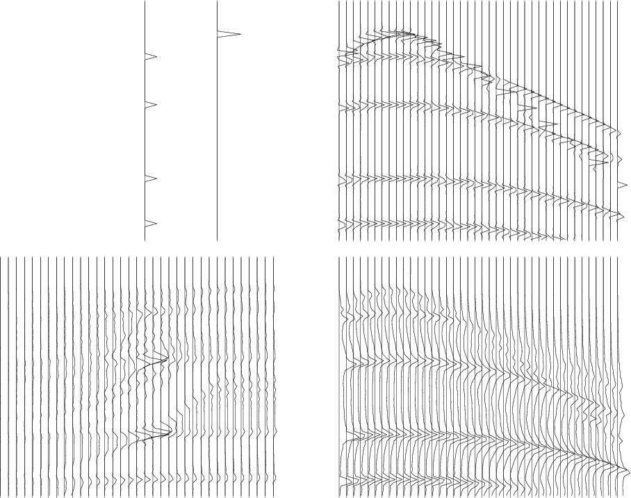
Figure 4.7 illustrates this smoothing by starting
from points in velocity space, transforming to offset,
and then back and forth again.
I omit that,
thus getting smoother results than theoretically preferable.
Figure 4.7 illustrates this smoothing by starting
from points in velocity space, transforming to offset,
and then back and forth again.
|
|---|
|
velvel
Figure 7. Iteration between spaces. Left are model spaces. Right are data spaces. Right derived from left. Lower model space derived from upper data space. |
|
|
There is one final complication relating to weighting.
The most symmetrical approach is to put
![]() into both
into both ![]() and
and ![]() .
Thus, because of the weighting by
.
Thus, because of the weighting by ![]() ,
the synthetic data in Figure 4.7 is
nonphysical.
An alternate view is to define
,
the synthetic data in Figure 4.7 is
nonphysical.
An alternate view is to define ![]() (by the pseudo code above, or by some modeling theory)
and then for reverse transformation
use
(by the pseudo code above, or by some modeling theory)
and then for reverse transformation
use ![]() .
.
An example is shown in Figure 4.8.

|
|---|
|
mutvel
Figure 8. Transformation of data as a function of offset (left) to data as a function of slowness (velocity scans) on the right using subroutine velsimp(). |
|
|
|
|
|
|
Moveout, velocity, and stacking |