Noncausal $f$ -$x$ -$y$ regularized nonstationary prediction filtering for random noise attenuation on 3D seismic data

f-x-y NRNA for random noise attenuation

Two dimensional $f$ -$x$ NRNA only considers one space coordinate x. If we use $f$ -$x$ NRNA on 3D seismic cube, we usually apply $f$ -$x$ RNA in one space slice. $f$ -$x$ NRNA reduces the effectiveness because the plane event in 3D cube is predictable along different directions rather than only one direction. Therefore, we should develop 3D $f$ -$x$ -$y$ NRNA to suppress random noise for 3D seismic data.

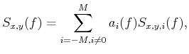
fig1
Figure 1. The $f$ -$x$ -$y$ prediction filter. The trace ${{\text {T}}_{\text {33}}}$ is predicted from circumjacent traces ${{\text {T}}_{11}}\sim {{\text {T}}_{55}}$ (except itself ${{\text {T}}_{\text {33}}}$ ).

Next, we use Fig. 1 to illustrate the idea of $f$ -$x$ -$y$ NRNA. The middle trace ${{\text {T}}_{\text {33}}}$ is the one we want to predict. Trace ${{\text {T}}_{\text {33}}}$ can be predicted from circumjacent traces ${{\text {T}}_{11}}\sim {{\text {T}}_{55}}$ (except itself ${{\text {T}}_{\text {33}}}$ ). The prediction process includes all different directions. For example, if we use ${{\text{T}}_{21}}$ to predict ${{\text {T}}_{\text {33}}}$ , we can estimate a corresponding coefficient using the described algorithm in the following. $f$ -$x$ -$y$ NRNA uses all around traces to predict the middle trace. Therefore, the prediction uses more information than $f$ -$x$ NRNA. For all the traces in 3D cube, similar to the trace ${{\text {T}}_{\text {33}}}$ , we can use circumjacent traces to predict them. Mathematically, we can write the prediction process as

$${{S}_{x,y}}(f)=\sum\limits_{i=-M,i\ne 0}^{M}{{{a}_{i}}(f){{S}_{x,y,i}}(f)},$$ (4)

where M and i are the number and index of circumjacent traces, respectively. In the case of Fig. 1, M=24 and i is from 1 to 24. Note that ${{S}_{x,y,i}}(f)$ indicates the 24 circumjacent traces around ${{S}_{x,y}}(f)$ . Eq. 4 is the equations of noncausal regularized stationary autoregression. Similarly to $f$ -$x$ NRNA, considerng the nonstationary case, we can obtain

$${{\tilde{S}}_{x,y}}(f)=\sum\limits_{i=-M,i\ne 0}^{M}{{{a}_{x,y,i}}(f){{S}_{x,y,i}}(f)},$$ (5)

where ${{a}_{x,y,i}}(f)$ is the space-varying coefficients, which means they have three free degrees, space axis x, space axis y and shift axis i. ${{\tilde{S}}_{x,y}}(f)$ can be regarded as the estimation of noise-free signal. However, the coefficients ${{a}_{x,y,i}}(f)$ are not known. Once we obtain the coefficients, we can estimate the effective signal using Eq. 5 Similar to $f$ -$x$ NRNA, we use shaping regularization to solve this ill-posed problem. Here, we assume that the coefficients ${{a}_{x,y,i}}(f)$ $f$ -$x$ -$y$ RNA are smooth along two space axes x and y, which is reasonable because the curved surface event in 3D seismic data is locally plane. Therefore, we can obtain the following least square problem with shaping regularization

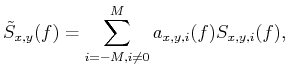
$$\min_{a_{x,y,i}(f)}\vert\vert{{S}_{x,y}}(f)-\sum\limits_{i=-M,i\ne 0}^{M}{{{a}_{x,y,i}}(f){{S}_{x,y,i}}(f)}\vert\vert _{2}^{2}+R[{{a}_{x,y,i}}(f)],$$ (6)

where R[.] denotes shaping regularization term which constrains coefficients ${{a}_{x,y,i}}(f)$ to be smooth along space axes. We use one coefficient with a given frequency and a given shift (e.g., from ${{\text{T}}_{21}}$ to ${{\text{T}}_{33}}$ indicated by arrow in Fig. 1) to explain the constraint in Eq. 6. This 3D cube of coefficient with a given frequency and a given shift can be expressed as ${{a}_{x,y,{{i}_{0}}}}({{f}_{0}})$ , which is smooth along with variables x and y. The smooth constraint of coefficients is the objective of shaping regularization. Finally, we use Eq. 6 to obtain obtain the complex coefficients of $f$ -$x$ -$y$ RNA, and use Eq. 5 to achieve the estimation of signal.

Transform-base methods can also be used for seismic noise attenuation (Ma and Plonka, 2010). Tang and Ma (1991) proposed to total-variation-based curvelet shrinkage for 3D seismic data denoising in order to suppress nonsmooth artifacts caused by the curvelet transform. Because the $f$ -$x$ -$y$ NRNA method uses shaping regularization to solve the ill-posed inverse problem and is complemented in frequency domain, it has higher computation efficiency than curvelet-based methods.

Noncausal $f$ -$x$ -$y$ regularized nonstationary prediction filtering for random noise attenuation on 3D seismic data