|
|
|
|
Stereographic imaging condition for wave-equation migration |
Wavefield reconstruction forms solutions to the considered (acoustic)
wave-equation with recorded data as boundary condition. We can
consider many different numeric solutions to the acoustic
wave-equation, which are distinguished, for example, by implementation
domain (space-time, frequency-wavenumber, etc.) or type of numeric
solution (differential, integral, etc.). Irrespective of numeric
implementation, we reconstruct two wavefields, one forward-propagated
from the source and one backward-propagated from the receiver
locations. Those wavefields can be represented as four-dimensional
objects function of position in space
![]() and time
and time ![]()
The second migration component is the imaging condition which is
designed to extract from the extrapolated wavefields (![]() and
and ![]() )
the locations where reflectors occur in the subsurface. The image
)
the locations where reflectors occur in the subsurface. The image
![]() can be extracted from the extrapolated wavefields by evaluating
the match between the source and receiver wavefields at every location
in the subsurface. The wavefield match can be evaluated using an
extended imaging condition
(Sava and Fomel, 2006,2005), where image
can be extracted from the extrapolated wavefields by evaluating
the match between the source and receiver wavefields at every location
in the subsurface. The wavefield match can be evaluated using an
extended imaging condition
(Sava and Fomel, 2006,2005), where image ![]() represents an estimate of the similarity between the source and
receiver wavefields in all
represents an estimate of the similarity between the source and
receiver wavefields in all ![]() dimensions, space (
dimensions, space (![]() ) and time
(
) and time
(![]() ):
):


|
|---|
|
velo,refl,dd
Figure 1. Constant velocity model (a), reflectivity model (b), data (c) and shot locations at |
|
|


|
|---|
|
velo,refl,dd
Figure 2. Velocity model with a negative Gaussian anomaly (a), reflectivity model (b), data (c) and shot location at |
|
|
The four-dimensional cross-correlation 3 maximizes at zero lag
if the source and receiver wavefields are correctly reconstructed. If
this is not true, either because we are using an approximate
extrapolation operator (e.g. one-way extrapolator with limited angular
accuracy), or because the velocity used for extrapolation is
inaccurate, the four-dimensional cross-correlation does not maximize
at zero lag and part of the cross-correlation energy is smeared over
space and time lags (
![]() and
and ![]() ). Therefore, extended imaging
conditions can be used to evaluate imaging accuracy, for example by
decomposition of reflectivity function of scattering angle at every
image location
(Sava and Fomel, 2006,2003; Biondi and Symes, 2004).
Angle-domain images carry information useful for migration velocity
analysis
(Sava and Biondi, 2004a; Shen et al., 2005; Biondi and Sava, 1999; Sava and Biondi, 2004b),
or for amplitude analysis
(Sava et al., 2001), or for attenuation of multiples
(Sava and Guitton, 2005; Artman et al., 2007)
). Therefore, extended imaging
conditions can be used to evaluate imaging accuracy, for example by
decomposition of reflectivity function of scattering angle at every
image location
(Sava and Fomel, 2006,2003; Biondi and Symes, 2004).
Angle-domain images carry information useful for migration velocity
analysis
(Sava and Biondi, 2004a; Shen et al., 2005; Biondi and Sava, 1999; Sava and Biondi, 2004b),
or for amplitude analysis
(Sava et al., 2001), or for attenuation of multiples
(Sava and Guitton, 2005; Artman et al., 2007)
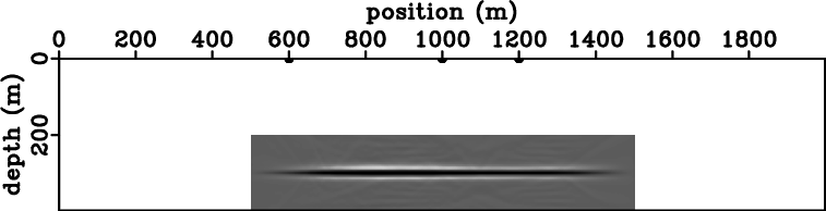
The conventional imaging condition 4 is the focus of this paper. As discussed above, assuming accurate extrapolation, this imaging condition should produce accurate images at zero cross-correlation lags. However, this conclusion does not always hold true, as illustrated next.
Figures 1(a) and 1(b) represent a simple model of
constant velocity with a horizontal reflector. Data in this model are
simulated from ![]() sources triggered simultaneously at coordinates
sources triggered simultaneously at coordinates
![]() m. Using the standard imaging procedure outlined in
the preceding paragraphs, we can reconstruct the source and receiver
wavefields,
m. Using the standard imaging procedure outlined in
the preceding paragraphs, we can reconstruct the source and receiver
wavefields, ![]() and
and ![]() , and apply the conventional imaging
condition equation 4 to obtain the image in Figure 3(a). The image
shows the horizontal reflector superposed with linear artifacts of
comparable strength.
, and apply the conventional imaging
condition equation 4 to obtain the image in Figure 3(a). The image
shows the horizontal reflector superposed with linear artifacts of
comparable strength.
Figures 2(a) and 2(b) represent another simple model
of spatially variable velocity with a horizontal reflector. Data in
this model are simulated from a source located at coordinate
![]() m. The negative Gaussian velocity anomaly present in the
velocity model creates triplications of the source and receiver
wavefields. Using the same standard imaging procedure outlined in the
preceding paragraphs, we obtain the image in Figure 5(a). The image
also shows the horizontal reflector superposed with complex artifacts
of comparable strength.
m. The negative Gaussian velocity anomaly present in the
velocity model creates triplications of the source and receiver
wavefields. Using the same standard imaging procedure outlined in the
preceding paragraphs, we obtain the image in Figure 5(a). The image
also shows the horizontal reflector superposed with complex artifacts
of comparable strength.
In both cases discussed above, the velocity model is perfectly known and the acoustic wave equation is solved with the same finite-difference operator implemented in the space-time domain. Therefore, the artifacts are caused only by properties of the conventional imaging condition used to produce the migrated image and not by inaccuracies of wavefield extrapolation or of the velocity model.
The cause of artifacts is cross-talk between events present in the source and receiver wavefields, which are not supposed to match. For example, cross-talk can occur between wavefields corresponding to multiple sources, as illustrated in the example shown in Figures 1(a)-1(b), multiple branches of a wavefield corresponding to one source, as illustrate in the example shown in Figures 2(a)-2(b), events that correspond to multiple reflections in the subsurface, or multiple wave modes of an elastic wavefield, for example between PP and PS reflections, etc.

|
|---|
|
ii,kk
Figure 3. Images obtained for the model in Figures 1(a)-1(c) using the conventional imaging condition (a) and the stereographic imaging condition (b). |
|
|
|
|
|
|
Stereographic imaging condition for wave-equation migration |