|
|
|
|
Interferometric imaging condition for wave-equation migration |
The imaging procedure in equations 5-8 can be generalized for
imaging prestack (multi-offset) data (Figure 1(b)). The conventional
imaging procedure for this type of data consists of two steps
(Claerbout, 1985): wavefield simulation from the source location
to the image coordinates
![]() and wavefield reconstruction at image
coordinates
and wavefield reconstruction at image
coordinates
![]() from data recorded at receiver coordinates
from data recorded at receiver coordinates
![]() ,
followed by an imaging condition evaluating the match between the
simulated and reconstructed wavefields.
,
followed by an imaging condition evaluating the match between the
simulated and reconstructed wavefields.
Let
![]() be the source wavefield constructed from the
location of the seismic source and
be the source wavefield constructed from the
location of the seismic source and
![]() the receiver
wavefield reconstructed from the receiver locations. A conventional
imaging procedure produces a seismic image as the zero-lag of the time
cross-correlation between the source and receiver
wavefields. Mathematically, we can represent this operation as
the receiver
wavefield reconstructed from the receiver locations. A conventional
imaging procedure produces a seismic image as the zero-lag of the time
cross-correlation between the source and receiver
wavefields. Mathematically, we can represent this operation as
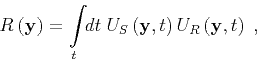 |
(9) |
When imaging in random media, the data recorded at the surface incorporates phase delays caused by the velocity variations encountered while waves propagate in the subsurface. In a typical seismic experiment, random phase delays accumulate both on the way from the source to the reflectors, as well as on the way from the reflectors to the receivers. Therefore, the receiver wavefield reconstructed using the background velocity model is characterized by random fluctuations, similar to the ones seen for wavefields reconstructed in the zero-offset situation. In contrast, the source wavefield is simulated in the background medium from a known source position and, therefore, it is not affected by random fluctuations. However, the zero-lag of the cross-correlations between the source wavefields (without random fluctuations) and the receiver wavefield (with random fluctuations), still generates image artifacts similar to the ones encountered in the zero-offset case.
Statistically stable imaging using pseudo WDFs can be obtained in this
case, too. What we need to do is attenuate the phase errors in the
reconstructed receiver wavefield and then apply a conventional imaging
condition. Therefore, a multi-offset interferometric imaging condition
can be formulated as
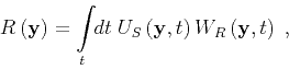 |
(10) |
|
|
|
|
Interferometric imaging condition for wave-equation migration |