 |
 |
 |
 | Isotropic angle-domain elastic reverse-time migration |  |
![[pdf]](icons/pdf.png) |
Next: Imaging with vector displacements
Up: Yan and Sava: Angle-domain
Previous: Vector wavefields
We test the different imaging conditions discussed in the preceding
sections with data simulated on a modified subset of the Marmousi II
model (Martin et al., 2002). The section is chosen to be at the left
side of the entire model which is relatively simple, and therefore it
is easier to examine the quality of the images.
|
|---|
vp,rx
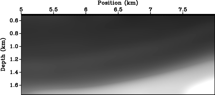
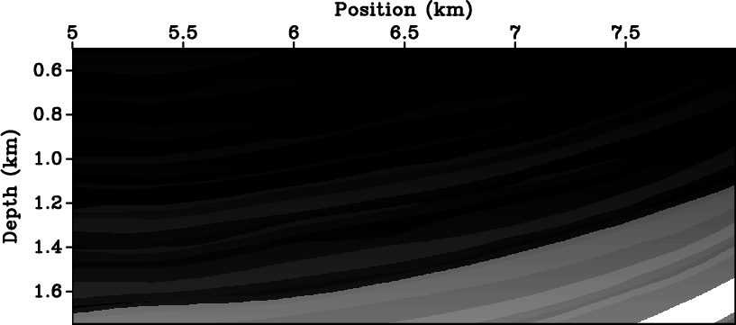
Figure 3. (a) P- and S-wave
velocity models and (b) density model used for isotropic elastic
wavefield modeling, where  ranges from ranges from  to to  km/s from
top to bottom and km/s from
top to bottom and  , and density ranges from , and density ranges from  to to
 g/cm g/cm . .
|
|---|
![[png]](icons/viewmag.png) ![[scons]](icons/configure.png)
|
|---|
|
|---|
de1,de2,df1,df2
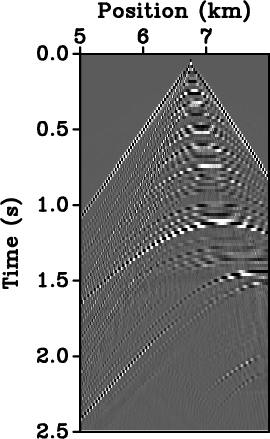
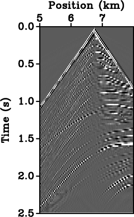
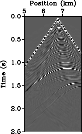
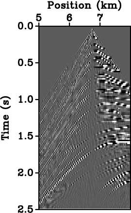
Figure 4. Elastic
data simulated in model 3a and 3b
with a source at  km and km and  km, and receivers at
km: (a) vertical component, (b) horizontal component, (c)
scalar potential and (d) vector potential of the elastic
wavefield. Both vertical and horizontal components, panels (a) and
(b), contain a mix of P and S modes, as seen by comparison with
panels (c) and (d). km, and receivers at
km: (a) vertical component, (b) horizontal component, (c)
scalar potential and (d) vector potential of the elastic
wavefield. Both vertical and horizontal components, panels (a) and
(b), contain a mix of P and S modes, as seen by comparison with
panels (c) and (d).
|
|---|
|
|
|---|
|
|---|
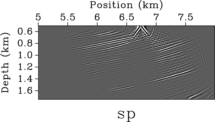
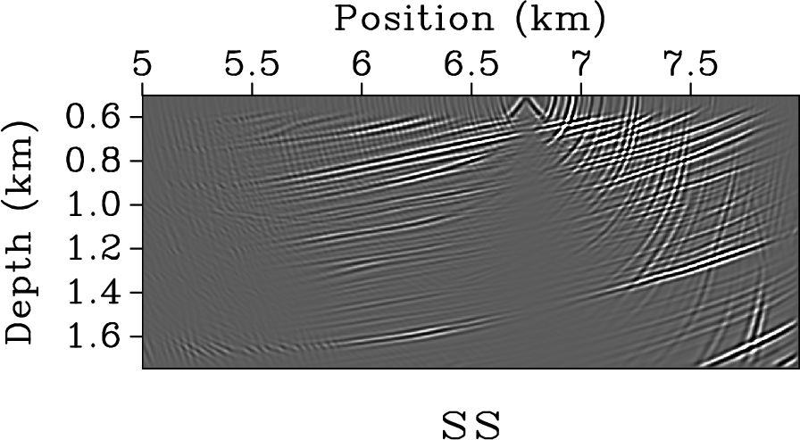
ieall0,ieall1,ieall2,ieall3
Figure 5. Images produced with the displacement components imaging
condition from equation ![[*]](icons/crossref.png) . Panels (a), (b), (c)
and (d) correspond to the cross-correlation of the
vertical and horizontal components of the source
wavefield with the vertical and horizontal components of
the receiver wavefield, respectively. Images (a) to (d)
are the . Panels (a), (b), (c)
and (d) correspond to the cross-correlation of the
vertical and horizontal components of the source
wavefield with the vertical and horizontal components of
the receiver wavefield, respectively. Images (a) to (d)
are the  , ,  , ,  and and  components,
respectively. The image corresponds to one shot at
position km and km. Receivers are located
at all locations at km. components,
respectively. The image corresponds to one shot at
position km and km. Receivers are located
at all locations at km.
|
|---|
|
|
|---|
|
|---|
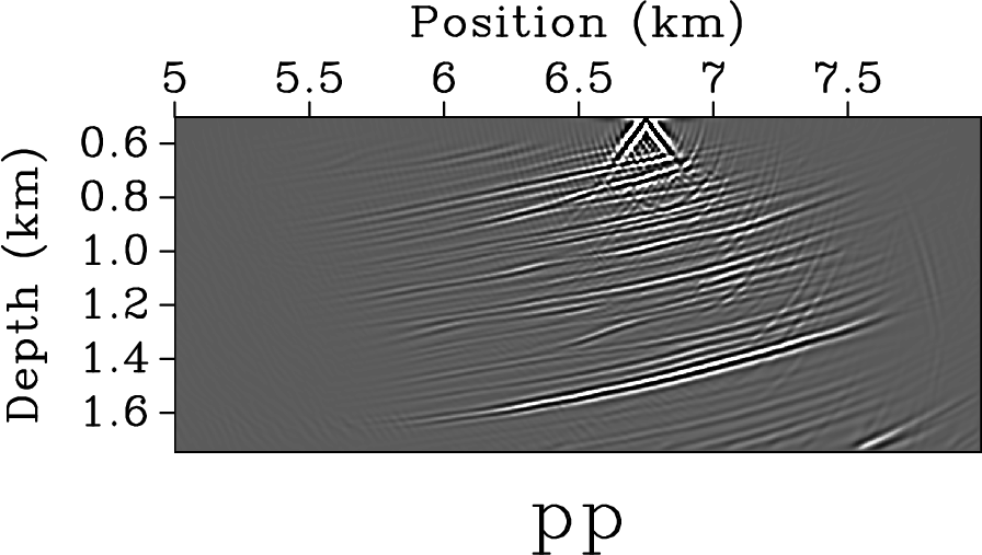
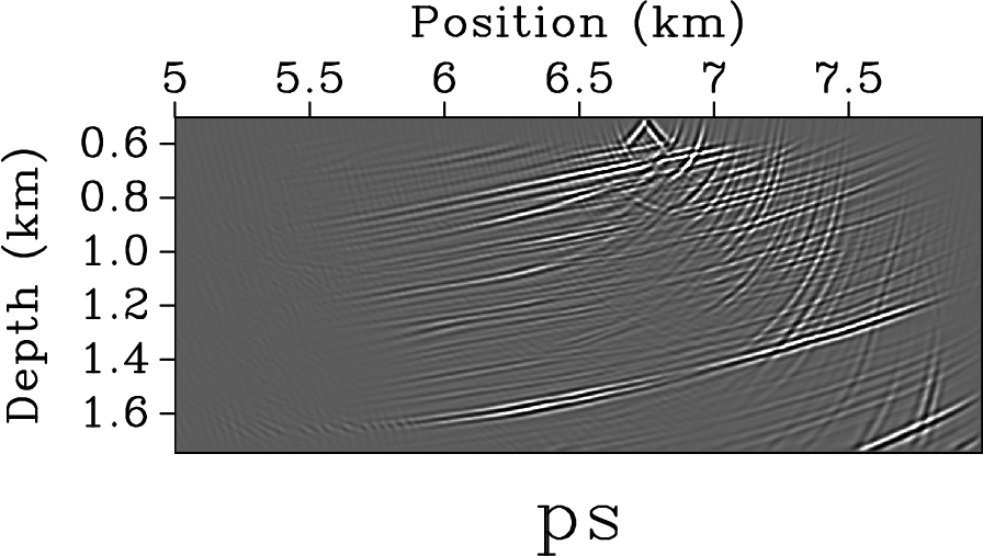
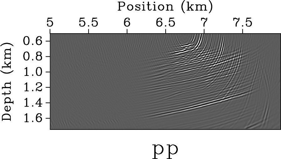
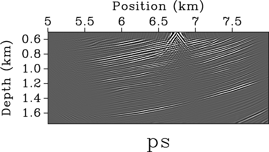
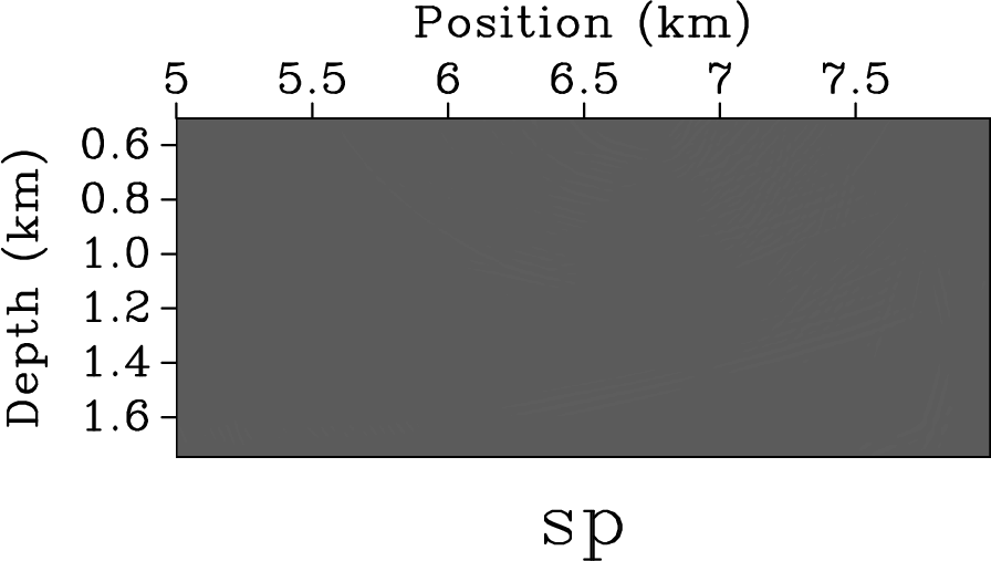
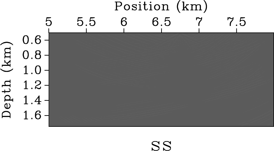
jeall0,jeall1,jeall2,jeall3
Figure 6. Images produced with the scalar and vector potentials
imaging condition from equation . Panels (a),
(b), (c) and (d) correspond to the cross-correlation of
the P and S components of the source wavefield with the
P and S components of the receiver wavefield,
respectively. Images (a) to (d) are the  , ,  , ,
 and and  components, respectively. The image
corresponds to one shot at position km and
km. Receivers are located at all locations at
km. Panels (c) and (d) are blank because
an explosive source was used to generate synthetic
data. components, respectively. The image
corresponds to one shot at position km and
km. Receivers are located at all locations at
km. Panels (c) and (d) are blank because
an explosive source was used to generate synthetic
data.
|
|---|
|
|
|---|
Subsections
|
|
|
|
| Isotropic angle-domain elastic reverse-time migration | |
|
Next: Imaging with vector displacements
Up: Yan and Sava: Angle-domain
Previous: Vector wavefields
2013-08-29