Numeric implementation of wave-equation migration velocity analysis operators

Mixed-domain operators

For the case of the phase-shift operation in media with lateral slowness variation, the mixed-domain solution involves forward and inverse Fourier transforms (denoted fFT and iFT in our algorithms) which can be implemented efficiently using standard Fast Fourier Transform algorithms. The numeric implementation is summarized in the following table:

In this chart, ${{k_z}^{{\bf k}}}$ denotes the $\omega -{\bf k}$ component of the depth wavenumber and ${{k_z}^{{\bf x}}}$ denotes the $\omega -{\bf x}$ component of the depth wavenumber. An example of mixed-domain implementation is the Split-Step Fourier (SSF) method, where ${{k_z}^{{\bf k}}}$ represents the SSR equation computed with a constant reference slowness $\tilde{s}$, and ${{k_z}^{{\bf x}}}=\omega \left (s-\tilde{s} \right)$ represents a space-domain correction (Stoffa et al., 1990).

Based on the equation 27, the derivative of the depth wavenumber relative to slowness is

$$\left. \frac{d {{k_z}}} {d s} \right\vert _{s_0} = \frac{\o... ...\vert}{ {\omega s} _0 \left ({\bf m}\right)} \right]^2} } \;.$$ (38)

The numeric implementation of the pseudo-differential equation A-1 is as complicated in media with lateral slowness variation as its phase-shift counterpart (equation 2). However, we can construct efficient and robust numeric implementations using similar approximations as the ones employed for the phase-shift relation, e.g. mixed-domain numeric implementation.

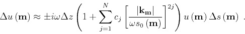
The linearized scattering operator can also be implemented in a mixed-domain by expanding the square-root from relation A-1 using a Taylor series expansion

$$\left. \frac{d {{k_z}}} {d s} \right\vert _{s_0} \approx \o... ... {\omega s} _0 \left ({\bf m}\right)} \right]^{2j} \right)\;,$$ (39)

where $c_j$ are binomial coefficients of the Taylor series.

Therefore, the wavefield perturbation at depth $z$ caused by a slowness perturbation at depth $z$ under the influence of the background wavefield at the same depth $z$ (forward scattering operator 8) can be written as

$${\Delta {u}} \left ({\bf m}\right)\approx \pm i\omega \Delta... ...ht){u} \left ({\bf m}\right)\Delta s \left ({\bf m}\right)\;.$$ (40)

Similarly, the slowness perturbation at depth $z$ caused by a wavefield perturbation at depth $z$ under the influence of the background wavefield at the same depth $z$ (adjoint scattering operator 11) can be written as

$$\Delta s \left ({\bf m}\right)\approx \mp i\omega \Delta z\left (... ...ight)\overline{{u} \left ({\bf m}\right)} {\Delta {u}} \left ({\bf m}\right)\;.$$ (41)

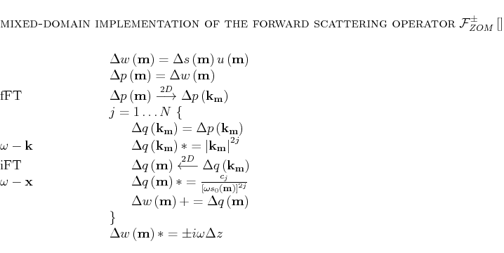
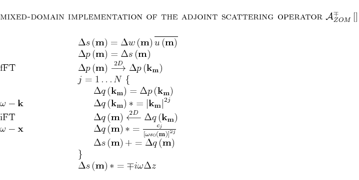
The mixed-domain implementation of the forward and adjoint scattering operators A-3 and A-4, is summarized on the following tables:

Numeric implementation of wave-equation migration velocity analysis operators