|
|
|
|
Numeric implementation of wave-equation migration velocity analysis operators |
The conceptual framework of wave-equation MVA is similar to that of conventional (ray-based) MVA in that the source of information for velocity updating is extracted from features of migrated images. This is in contrast with wave-equation tomography (or inversion), where the source of information is represented by the mismatch between recorded and simulated data. The main difference between wave-equation MVA and ray-based MVA is that the carrier of information from the migrated images to the velocity model is represented by the entire extrapolated wavefield and not by a rayfield constructed from selected points in the image based on an approximate velocity model.
The key element for the wave-equation MVA technique is a definition of an image perturbation corresponding to the difference between the image obtained with a known background velocity model and an improved image. Such image perturbations can be constructed using straight differences between images (Albertin et al., 2006a; Biondi and Sava, 1999), or by examining moveout parameters in migrated images (Shen et al., 2005; Sava and Biondi, 2004a; Maharramov and Albertin, 2007; Albertin et al., 2006b; Sava and Biondi, 2004b). Then, using wave-equation MVA operators, the image perturbations can be translated into slowness perturbations which update the model. The direct analogy between wave-based MVA and ray-based MVA is the following: wave-based methods use image perturbations and back-propagation using waves, while ray-based methods use traveltime perturbations and back-propagation using rays. Thus, wave-equation MVA benefits from all the characteristics of wave-based imaging techniques, e.g. stability in areas of large velocity variation, while remaining conceptually similar to conventional traveltime-based MVA.
We can formulate wave-equation migration and velocity analysis for different configurations in which we process the recorded data. There are two main classes of wave-equation migration, survey-sinking migration and shot-record migration (Claerbout, 1985), which differ in the way in which recorded data are processed. Both wave-equation imaging techniques use similar algorithms for downward continuation and, in theory, produce identical images for identical implementation of extrapolation operators and if all data are used for imaging (Berkhout, 1982; Biondi, 2003). The main difference is that shot-record migration is used to process separate seismic experiments (shots) sequentially, while survey-sinking migration is used to process all seismic experiments (shots) simultaneously. The shot-record operators are more computationally expensive but less memory intensive than the survey-sinking operators. A special case of survey-sinking migration assumes the sources and receivers are coincident on the acquisition surface, a technique usually described as the exploding reflector model (Loewenthal et al., 1976) applicable to zero-offset data. All operators described here can be used in models characterized by complex wave propagation (multipathing).
In all situations, wave-equation migration can be formulated as
consisting of two main steps. The first step is wavefield
reconstruction (abbreviated
![]() for the rest of this paper) at
all locations in space and using all frequencies from the recorded
data as boundary conditions. This step requires numeric solutions to a
form of wave equation, typically the one-way acoustic wave
equation. The second step is the imaging condition (abbreviated
for the rest of this paper) at
all locations in space and using all frequencies from the recorded
data as boundary conditions. This step requires numeric solutions to a
form of wave equation, typically the one-way acoustic wave
equation. The second step is the imaging condition (abbreviated
![]() for the rest of this paper), which is used to extract from the
reconstructed wavefield(s) the locations where reflectors occur. This
step requires numeric implementation of image processing techniques,
e.g. cross-correlation, which evaluate properties of the wavefield
indicating the presence of reflectors. Needless to say, the two steps
are not implemented sequentially in practice, since the size of the
wavefield is usually large and cannot be handled efficiently on
conventional computers. Instead, wavefield reconstruction and imaging
condition are implemented on-the-fly, avoiding expensive data storage
and retrieval. Wave-equation MVA requires implementation of an
additional procedure which links image and slowness
perturbations. This link is given by a wavefield scattering
operation (abbreviated
for the rest of this paper), which is used to extract from the
reconstructed wavefield(s) the locations where reflectors occur. This
step requires numeric implementation of image processing techniques,
e.g. cross-correlation, which evaluate properties of the wavefield
indicating the presence of reflectors. Needless to say, the two steps
are not implemented sequentially in practice, since the size of the
wavefield is usually large and cannot be handled efficiently on
conventional computers. Instead, wavefield reconstruction and imaging
condition are implemented on-the-fly, avoiding expensive data storage
and retrieval. Wave-equation MVA requires implementation of an
additional procedure which links image and slowness
perturbations. This link is given by a wavefield scattering
operation (abbreviated
![]() for the rest of this paper) which is
derived by linearization from conventional wavefield extrapolation
operators.
for the rest of this paper) which is
derived by linearization from conventional wavefield extrapolation
operators.
In the following sections, we describe the migration and velocity
analysis operators for the various imaging configurations. We begin
with zero-offset imaging under the exploding reflector model, because
this is the simplest wave-equation imaging framework and can aid our
understanding of both survey-sinking and shot-record migration and
velocity analysis frameworks. We then continue with a description of
the wave-equation migration velocity analysis operator for
multi-offset data using the survey-sinking and shot-record migration
configuration. For each configuration, we describe the implementation
of the forward operator (used to translate model perturbations
into image perturbations) and of the adjoint operator (used to
transform image perturbations into model perturbations). Both forward
and adjoint operators are necessary for the implementation of
efficient numeric conjugate gradient optimization
(Claerbout, 1985).
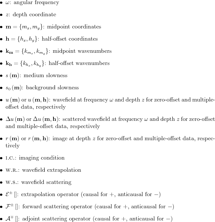
Throughout this paper, we are using the following notations and naming
conventions:
|
|
|
|
Numeric implementation of wave-equation migration velocity analysis operators |