 |
 |
 |
 | Numeric implementation of
wave-equation migration velocity analysis operators |  |
![[pdf]](icons/pdf.png) |
Next: Shot-record migration and velocity
Up: Wave-equation migration and velocity
Previous: Zero-offset migration and velocity
Wavefield reconstruction for multi-offset migration based on the
one-way wave-equation under the survey-sinking framework
(Claerbout, 1985) is implemented similarly to the zero-offset
case by recursive phase-shift of prestack wavefields
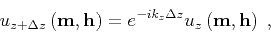 |
(12) |
followed by extraction of the image at time  . Here,
  and
and
 stand for midpoint and half-offset coordinates, respectively,
defined according to the relations
stand for midpoint and half-offset coordinates, respectively,
defined according to the relations
where  and
and  are coordinates of sources and receivers on the
acquisition surface. In equation 12,
are coordinates of sources and receivers on the
acquisition surface. In equation 12,
 represents the
acoustic wavefield for a given frequency
represents the
acoustic wavefield for a given frequency  at all midpoint
positions and half-offsets at depth
at all midpoint
positions and half-offsets at depth  , and
, and
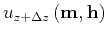 represents the same wavefield extrapolated to depth
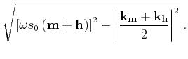
 . The phase shift operation uses the depth wavenumber
  which is defined by the double square-root (DSR) equation
The image is obtained from this extrapolated wavefield by selection of
time , which is usually implemented as summation over
frequencies:
 |
(16) |
Similarly to the derivation done in the zero-offset case, we can
assume the separation of the extrapolation slowness
 into a
background component
into a
background component
 and an unknown perturbation component
 . Then we can construct a wavefield perturbation
 at depth and frequency related linearly to the slowness
perturbation
. Linearizing the depth wavenumber given by the
DSR equation 15 relative to the background slowness
,
we obtain
at depth and frequency related linearly to the slowness
perturbation
. Linearizing the depth wavenumber given by the
DSR equation 15 relative to the background slowness
,
we obtain
 |
(17) |
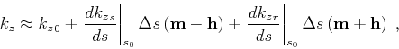
where the depth wavenumber in the background medium is
Here,
represents the spatially-variable background
slowness at depth level . Using the wavenumber linearization given
by equation 17, we can reconstruct the acoustic wavefields in the
background model using a phase-shift operation
 |
(19) |
We can represent wavefield extrapolation using a generic solution to
the one-way wave-equation using the notation
![${u}_{z+\Delta z}\left ({\bf m},{\bf h}\right)= \mathcal{E}^{-}_{SSM}\left [{s_0}_z \left ({\bf m}\right),{u}_z\left ({\bf m},{\bf h}\right) \right]$](img74.png) . This
notation indicates that the wavefield
is
reconstructed from the wavefield
using the background
slowness
. This operation is repeated independently for all
frequencies . A typical implementation of survey-sinking
wave-equation migration uses the following algorithm:
. This
notation indicates that the wavefield
is
reconstructed from the wavefield
using the background
slowness
. This operation is repeated independently for all
frequencies . A typical implementation of survey-sinking
wave-equation migration uses the following algorithm:
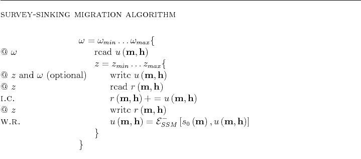
This algorithm is similar to the one described in the preceding
section for zero-offset migration, except that the wavefield and image
are parametrized by midpoint and half-offset coordinates and that the
depth wavenumber used in the extrapolation operator is given by the
DSR equation using the background slowness
. Wavefield
extrapolation is usually implemented in a mixed domain
(space-wavenumber), as briefly summarized in Appendix A.
Similarly to the derivation of the wavefield perturbation in the
zero-offset migration case, we can write the linearized wavefield
perturbation for survey-sinking migration as
Equation 20 defines the forward scattering operator
![$ \mathcal{F}^{-}_{SSM}\left [{u}\left ({\bf m},{\bf h}\right),s_0 \left ({\bf m}\right),\Delta s\left ({\bf m},{\bf h}\right) \right]$](img83.png) , producing the scattered
wavefield
from the slowness perturbation
, based
on the background slowness
and background wavefield
, producing the scattered
wavefield
from the slowness perturbation
, based
on the background slowness
and background wavefield
 . The image perturbation at depth is obtained from the
scattered wavefield using the time imaging condition, similar to
the procedure used for imaging in the background medium:
. The image perturbation at depth is obtained from the
scattered wavefield using the time imaging condition, similar to
the procedure used for imaging in the background medium:
 |
(21) |
Given an image perturbation
 , we can construct the scattered
wavefield by the adjoint of the imaging condition
, we can construct the scattered
wavefield by the adjoint of the imaging condition
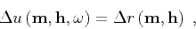 |
(22) |
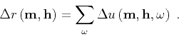
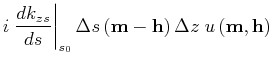
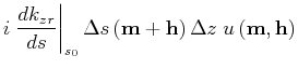
for every frequency . Then, similarly to the procedure used in
the zero-offset case, the slowness perturbation at depth caused by
a wavefield perturbation at depth under the influence of the
background wavefield at the same depth can be written as
and
Equations 23-24 define the adjoint scattering operator
![$ \mathcal{A}^{+}_{SSM}\left [{u}\left ({\bf m},{\bf h}\right),s_0 \left ({\bf m}\right),{\Delta {u}}\left ({\bf m},{\bf h}\right) \right]$](img94.png) , producing the slowness
perturbation
from the scattered wavefield
, based
on the background slowness
and background wavefield
. A typical implementation of survey-sinking forward and
adjoint scattering follows the algorithms:
, producing the slowness
perturbation
from the scattered wavefield
, based
on the background slowness
and background wavefield
. A typical implementation of survey-sinking forward and
adjoint scattering follows the algorithms:
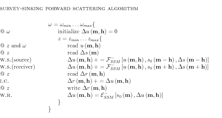
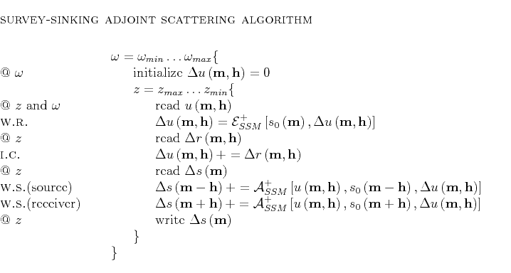
These algorithms are similar to the ones described in the preceding
section for zero-offset migration, except that the wavefield and image
are parametrized by midpoint and half-offset coordinates.
Furthermore, the two square-roots corresponding to the DSR equation
update the slowness model separately, thus characterizing the source
and receiver propagation paths to the image positions.
Both forward and adjoint scattering algorithms require the background
wavefield,
, to be precomputed at all depth levels.
Scattering and wavefield extrapolation are implemented in the mixed
space-wavenumber domain, as briefly explained in Appendix A.
|
|
|
|
| Numeric implementation of
wave-equation migration velocity analysis operators | |
|
Next: Shot-record migration and velocity
Up: Wave-equation migration and velocity
Previous: Zero-offset migration and velocity
2013-08-29

![$\displaystyle \sqrt{ \left [{ {\omega s} _0\left ({\bf m}-{\bf h}\right)} \right]^2 - \left\vert {\frac{{{\bf k}_{\bf m}}-{{\bf k}_{\bf h}}}{2}} \right\vert^2}$](img71.png)
![$\displaystyle \sqrt{ \left [{ {\omega s} \left ({\bf m}-{\bf h}\right)} \right]^2 - \left\vert {\frac{{{\bf k}_{\bf m}}-{{\bf k}_{\bf h}}}{2}} \right\vert^2}$](img64.png)
![$\displaystyle \sqrt{ \left [{ {\omega s} \left ({\bf m}+{\bf h}\right)} \right]^2 - \left\vert {\frac{{{\bf k}_{\bf m}}+{{\bf k}_{\bf h}}}{2}} \right\vert^2} \;.$](img66.png)
![$\displaystyle i\Delta z \frac{\omega {u}\left ({\bf m},{\bf h}\right)\Delta s\l...
...bf h}}} \right\vert}{2 {\omega s} _0\left ({\bf m}-{\bf h}\right)} \right]^2} }$](img81.png)
![$\displaystyle i\Delta z \frac{\omega {u}\left ({\bf m},{\bf h}\right)\Delta s\l...
...}}} \right\vert}{2 {\omega s} _0\left ({\bf m}+{\bf h}\right)} \right]^2} } \;.$](img82.png)
![$\displaystyle i\Delta z \frac{\omega \overline{{u}\left ({\bf m},{\bf h}\right)...
...}}} \right\vert}{2 {\omega s} _0\left ({\bf m}-{\bf h}\right)} \right]^2} } \;,$](img90.png)

![$\displaystyle i\Delta z \frac{\omega \overline{{u}\left ({\bf m},{\bf h}\right)...
...}}} \right\vert}{2 {\omega s} _0\left ({\bf m}+{\bf h}\right)} \right]^2} } \;.$](img93.png)