Open Data/Open Source: Seismic Unix scripts to process a 2D land line

Data Loading and initial data QC

I found little documentation about loading data and creating trace headers in previous publications. This section described how I loaded the headers.

The three field data SEGY files are downloaded, converted to Seismic Unix format, concatenated, and a print created of the range of each trace header using the command:

scons list1.su

Or to use the tar file type:

./list1.job

The resulting listing is:

6868 traces:
tracl    1 6868 (1 - 6868)
tracr    1 6868 (1 - 6868)
fldr     101 168 (101 - 168)
tracf    1 101 (1 - 101)
trid     1
ns       3000
dt       2000
f1       0.000000 512.000000 (0.000000 - 512.000000)

The print indicates there is little information in the input headers. There are 31 shot records (fldr 101 - 130) and each record has 101 traces (tracf 1 - 101). The trace headers will be created using fldr (the field record number) and tracf (the field trace number). A list of these headers on the first 3000 traces is created using:

scons list2.su

If you are using the tar file type:

./list2.job

Part of the print is:

fldr=101 tracf=1  cdp=0	 cdpt=0  offset=0 
fldr=101 tracf=2  cdp=0	 cdpt=0  offset=0 	
fldr=101 tracf=3  cdp=0  cdpt=0  offset=0 
... 
fldr=101 tracf=101  cdp=0  cdpt=0  offset=0 
fldr=102 tracf=1    cdp=0  cdpt=0  offset=0 
fldr=102 tracf=2    cdp=0  cdpt=0  offset=0 
...

A first display of the seismic data and a zoom of the same data (figures 3 and 4) are produced with the commands:

scons first.view 
scons zoomfirst.view

If you are using the tar file type:

./first.job
./zoomfirst.job

first
Figure 3. First 3000 traces on the first SEGY file.

zoomfirst
Figure 4. Zoom of Figure 3. The first look at the data. Notice the ground roll and good signal. There are 101 traces in each shotpoint, 5 auxiliary traces and 96 data traces.

The first 10 records in the file are test records. These test records are the unusual traces in the left third of Figure 3. The Observer Log does not mention these test records, but indicates the first shotpoint is field file identifier (ffid) 110. There are also 5 auxiliary traces in each shot record. These auxiliary traces can be seen on Figure 4.

The display of shotpoint 24 (Figure 4) is displayed with the command:

scons firstrec24.view

If you are using the tar file type:

./firstrec24.job

This display as created using suwind to select traces 2324 through 2424, so it is the 24th record in the input file (including the test records). This plot confirms that the 5 auxiliary traces are tracf 97 through 101.

firstrec24
Figure 5. The 24th shot record without processing. The last 5 traces traces are auxiliary traces. There is noise on the traces closest to the shotpoint. One trace has a noise burst near the maximum time.

The movie display is not included in this paper. The movie loops continuously and can be stopped by pressing 's'. Once stopped, you can move forward or backward using the 'f' and 'b' keys. The movie can be run with the command:

scons firstmovie.view

If you are using the tar file type:

./firstmovie.job

The trace headers are loaded using the command:

scons allshots.su

Or from the tar file:

./allshots.job

The stages in loading the trace header are

1. Run sugethw to create the file hdrfile.txt containing one record for each trace with tracl, fldr, tracf
2. Run the custom Python program InterpText.py. This program
   1. reads recnoSpn.txt that defines the recno/spn relationship
   2. reads spnElev.txt the defined the elevation of each shot
   3. interpolates this data and output hdrfile1.txt with values for all keys to be loaded
3. converts hdrfile1.txt to binary format (binary_hdrfile1.dat)
4. loads the trace headers
5. removes bad shotpoints and CDPs (with value=-999999)
6. removes the bad shotpoint 149
7. outputs allshots.su

InterpText.py is a custom Python script to load the trace headers. The code is not elegant, but it is straightforward and works. This program requires files to define the shotpoint elevation and the 'ffid'/'ep' relationship. The surveyor log defines the shotpoint elevations. The observers log describes the relationship between the su header keys 'ffid' and 'ep' (these are called 'REC' and 'SHOTPOINT' by in the observers log). This information was typed into two files (recnoSpn.txt and spnElev.txt). In addition to interpolating the record number/shotpoint table and the elevation data the program also computes the geometry including the receiver locations and the CDP numbers.

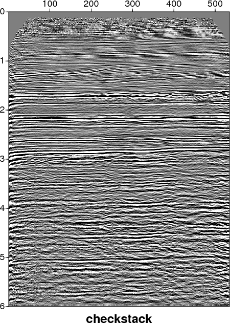
The stack file from the previous process is downloaded and displayed using the commands:

scons checkstack.view 
scons zoomcheckstack.view

If you are using the tar file type:

./checkstack.job
./zoomcheckstack.job

The first result is shown in Figure 6. The zoom display is not shown.

checkstack
Figure 6. Plot of the SEGY of the final stack from the 1981 processing.

Open Data/Open Source: Seismic Unix scripts to process a 2D land line