 |
 |
 |
 | Model fitting by least squares |  |
![[pdf]](icons/pdf.png) |
Next: OPERATOR SCALING (BINORMALIZATION)
Up: VESUVIUS PHASE UNWRAPPING
Previous: Estimating the inverse gradient
We have found a numerical solution to fitting applications, such as:
 |
(92) |
An analytical solution is much faster.
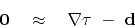
From any regression, we get the least
squares solution when we multiply by the transpose of the operator. Thus,
 |
(93) |
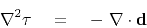
We need to understand what is the transpose of the gradient operator.
Recall the finite difference representation of a derivative in Chapter 1.
Ignoring end effects,
the transpose of a derivative is the negative of a derivative.
Because the transpose of a column vector is a row vector,
the adjoint of a gradient  , namely,
 is more commonly known as the vector divergence
(
is more commonly known as the vector divergence
( ).
Likewise,
).
Likewise,
 is a positive definite matrix,
the negative of the Laplacian
is a positive definite matrix,
the negative of the Laplacian  .
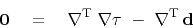
Thus, in more conventional mathematical notation,
the solution
.
Thus, in more conventional mathematical notation,
the solution  is that of Poisson's equation.
 |
(94) |
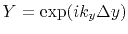
In the Fourier domain, we can have an analytic solution.
There,
 where
where  are the Fourier frequencies on the
  axes.
Instead of thinking
of equation (94) as a convolution in physical space,
think of it as a product in Fourier space.
Thus, the analytic solution is:
axes.
Instead of thinking
of equation (94) as a convolution in physical space,
think of it as a product in Fourier space.
Thus, the analytic solution is:
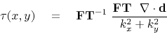 |
(95) |
where FT denotes two-dimensional Fourier transform over  and
and  .
Here is a trick from numerical analysis that gives better results: Instead of
representing the denominator
.
Here is a trick from numerical analysis that gives better results: Instead of
representing the denominator  in the most obvious way, let us represent it
in a manner consistent with the finite-difference way we expressed the numerator
in the most obvious way, let us represent it
in a manner consistent with the finite-difference way we expressed the numerator
 . Recall that
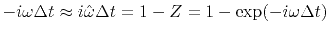 ,
which is a Fourier
domain way of saying that difference equations tend to differential equations at low
frequencies. Likewise, a symmetric second time derivative has a finite-difference
representation proportional to
,
which is a Fourier
domain way of saying that difference equations tend to differential equations at low
frequencies. Likewise, a symmetric second time derivative has a finite-difference
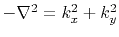
representation proportional to 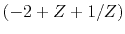 and in a two-dimensional space, a
finite-difference representation of the Laplacian operator is proportional to
and in a two-dimensional space, a
finite-difference representation of the Laplacian operator is proportional to
 , where
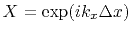 and
and
 .
Fourier solutions have peculiarities (periodic boundary conditions)
that are not always appropriate in practice, but having these solutions available
is often a nice place to start from when solving an application that cannot be solved
in Fourier space.
.
Fourier solutions have peculiarities (periodic boundary conditions)
that are not always appropriate in practice, but having these solutions available
is often a nice place to start from when solving an application that cannot be solved
in Fourier space.
For example, suppose we feel some data values are bad, and we
would like to throw out the regression equations involving the bad data points. At
Vesuvius, we might consider the strength of the radar return (which we have
previously ignored) and use it as a weighting function  .
Now, our regression (92) becomes:
.
Now, our regression (92) becomes:
 |
(96) |
which is a regression with an operator
 and
data
and
data  . The weighted problem is not solvable in the Fourier domain, because
the operator
. The weighted problem is not solvable in the Fourier domain, because
the operator
 has no simple
expression in the Fourier domain.
Thus,
we would use the analytic solution to the unweighted problem as a starting guess for
the iterative solution to the real problem.
has no simple
expression in the Fourier domain.
Thus,
we would use the analytic solution to the unweighted problem as a starting guess for
the iterative solution to the real problem.
With the Vesuvius data, we could construct a weight from the signal strength.
We also have available the curl, which should vanish.
Vanishing is an indicator of questionable data
that should be weighted down relative to other data.
|
|
|
|
| Model fitting by least squares | |
|
Next: OPERATOR SCALING (BINORMALIZATION)
Up: VESUVIUS PHASE UNWRAPPING
Previous: Estimating the inverse gradient
2014-12-01