Multidimensional autoregression

Adding noise (Geostat)

In chapter we restored missing data by adopting the philosopy of minimizing the energy in filtered output. In this chapter we learned about an optimum filter for this task, the prediction-error filter (PEF). Let us name this method the ``minimum noise'' method of finding missing data.

A practical application with the minimum-noise method is evident in a large empty hole such as in Figures 16- 17. In such a void the interpolated data diminishes greatly. Thus we have not totally succeeded in the goal of ``hiding our data acquisition footprint'' which we would like to do if we are trying to make pictures of the earth and not pictures of our data acquisition footprint.

What we will do next is useful in some applications but not in others. Misunderstood or misused it is rightly controversial. We are going to fill the empty holes with something that looks like the original data but really isn't. I will distinguish the words ``synthetic data'' (that derived from a physical model) from ``simulated data'' (that manufactured from a statistical model). We will fill the empty holes with simulated data like what you see in the center panels of Figures 3-9. We will add just enough of that ``wall paper noise'' to keep the variance constant as we move into the void.

Given some data $\bold d$ , we use it in a filter operator $\bold D$ , and as described with equation (29) we build a weighting function $\bold W$ that throws out the broken regression equations (ones that involve missing inputs). Then we find a PEF $\bold a$ by using this regression.

$$\bold 0 \quad\approx\quad \bold r \quad = \quad \bold W \bold D \bold a$$ (31)

Because of the way we defined $\bold W$ , the ``broken'' components of $\bold r$ vanish. We need to know the variance $\sigma$ of the nonzero terms. It can be expressed mathematically in a couple different ways. Let $\bold 1$ be a vector filled with ones and let $\bold r^2$ be a vector containing the squares of the components of $\bold r$ .

$$\sigma \quad = \quad \sqrt{ {1\over N} \sum_i^N r_i^2 } \quad = \quad \sqrt{ \bold 1' \bold W \bold r^2 \over \bold 1' \bold W \bold 1 }$$ (32)

Let us go to a random number generator and get a noise vector $\bold n$ filled with random numbers of variance $\sigma$ . We'll call this the ``added random noise''. Now we solve this new regression for the data space $\bold d$ (both known and missing)

$$\bold 0 \quad\approx\quad \bold r \quad = \quad \bold A \bold d - \bold n$$ (33)

keeping in mind that known data is constrained (as detailed in chapter ).

To understand why this works, consider first the training image, a region of known data. Although we might think that the data defines the white noise residual by $\bold r=\bold A\bold d$ , we can also imagine that the white noise determines the data by $\bold d=\bold A^{-1}\bold r$ . Then consider a region of wholly missing data. This data is determined by $\bold d=\bold A^{-1}\bold n$ . Since we want the data variance to be the same in known and unknown locations, naturally we require the variance of $\bold n$ to match that of $\bold r$ .

A very minor issue remains. Regression equations may have all of their required input data, some of it, or none of it. Should the $\bold n$ vector add noise to every regression equation? First, if a regression equation has all its input data that means there are no free variables so it doesn't matter if we add noise to that regression equation because the constraints will overcome that noise. I don't know if I should worry about how many inputs are missing for each regression equation.

It is fun making all this interesting ``wall paper'' noticing where it is successful and where it isn't. We cannot help but notice that it seems to work better with the genuine geophysical data than it does with many of the highly structured patterns. Geophysical data is expensive to acquire. Regrettably, we have uncovered a technology that makes counterfeiting much easier.

Examples are in Figures 16-19. In the electronic book, the right-side panel of each figure is a movie, each panel being derived from different random numbers.

herr-hole-fillr
Figure 16. The herringbone texture is a patchwork of two textures. We notice that data missing from the hole tends to fill with the texture at the edge of the hole. The spine of the herring fish, however, is not modeled at all.

brick-hole-fillr
Figure 17. The brick texture has a mortar part (both vertical and horizontal joins) and a brick surface part. These three parts enter the empty area but do not end where they should.

ridges-hole-fillr
Figure 18. The theoretical model is a poor fit to the ridge data since the prediction must try to match ridges of all possible orientations. This data requires a broader theory which incorporates the possibility of nonstationarity (space variable slope).

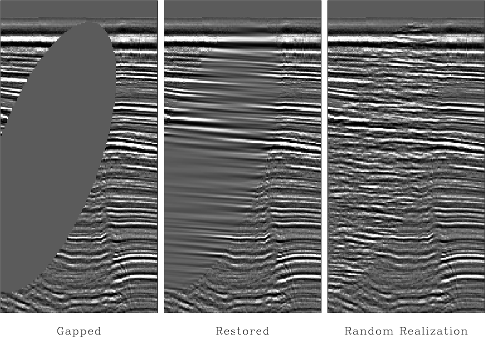
WGstack-hole-fillr
Figure 19. Filling the missing seismic data. The imaging process known as ``migration'' would suffer diffraction artifacts in the gapped data that it would not suffer on the restored data.

The seismic data in Figure 19 illustrates a fundamental principle: In the restored hole we do not see the same spectrum as we do on the other panels. This is because the hole is filled, not with all frequencies (or all slopes) but with those that are most predictable. The filled hole is devoid of the unpredictable noise that is a part of all real data.

Multidimensional autoregression