 |
 |
 |
 | Multidimensional autoregression |  |
![[pdf]](icons/pdf.png) |
Next: PREDICTION-ERROR FILTER OUTPUT IS
Up: Multidimensional autoregression
Previous: SOURCE WAVEFORM, MULTIPLE REFLECTIONS
Given  and
and  , you might like to predict
  .
Earliest application of the ideas in this chapter
came in the predictions of markets.
Prediction of a signal from its past is called ``autoregression'',
because a signal is regressed on itself ``auto''.
To find the scale factors you would optimize the fitting goal below,
for the prediction filter
.
Earliest application of the ideas in this chapter
came in the predictions of markets.
Prediction of a signal from its past is called ``autoregression'',
because a signal is regressed on itself ``auto''.
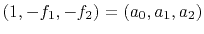
To find the scale factors you would optimize the fitting goal below,
for the prediction filter  :
:
![$\displaystyle \bold 0 \quad \approx \quad \bold r \eq \left[ \begin{array}{ccc}...
... - \left[ \begin{array}{c} y_2 \ y_3 \ y_4 \ y_5 \ y_6 \end{array} \right]$](img34.png) |
(9) |
(In practice, of course the system of equations would be
much taller, and perhaps somewhat wider.)
A typical row in the matrix (9)
says that
 hence the description of
  as a ``prediction'' filter.
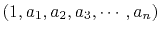
The error in the prediction is simply the residual.
Define the residual to have opposite polarity
and merge the column vector into the matrix, so you get
as a ``prediction'' filter.
The error in the prediction is simply the residual.
Define the residual to have opposite polarity
and merge the column vector into the matrix, so you get
![$\displaystyle \left[ \begin{array}{c} 0 \ 0 \ 0 \ 0 \ 0 \end{array} \right]...
...array} \right] \; \left[ \begin{array}{c} 1 \ -f_1 \ -f_2 \end{array} \right]$](img37.png) |
(10) |
which is a standard form for autoregressions and prediction error.
Multiple reflections
are predictable.
It is the unpredictable part of a signal,
the prediction residual,
that contains the primary information.
The output of the filter
 is the unpredictable part of the input.
This filter is a simple example of
a ``prediction-error'' (PE) filter.
It is one member of a family of filters called ``error filters.''
is the unpredictable part of the input.
This filter is a simple example of
a ``prediction-error'' (PE) filter.
It is one member of a family of filters called ``error filters.''
The error-filter family are filters with one coefficient constrained
to be unity and various other coefficients constrained to be zero.
Otherwise, the filter coefficients are chosen to have minimum power output.
Names for various error filters follow:
|
prediction-error (PE) filter |
|
gapped PE filter with a gap |
|
interpolation-error (IE) filter |
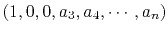
We introduce a
free-mask matrix  which ``passes'' the freely variable coefficients in the filter
and ``rejects'' the constrained coefficients
(which in this first example is merely the first coefficient
which ``passes'' the freely variable coefficients in the filter
and ``rejects'' the constrained coefficients
(which in this first example is merely the first coefficient  ).
).
![$\displaystyle \bold K \eq \left[ \begin{array}{cccccc} 0 & . & . \ . & 1 & . \ . & . & 1 \end{array} \right]$](img44.png) |
(11) |
To compute a simple prediction error filter
 with the CD method,
we write
(9) or
(10) as
with the CD method,
we write
(9) or
(10) as
![$\displaystyle \bold 0 \quad \approx \quad \bold r \eq \left[ \begin{array}{ccc}...
... + \left[ \begin{array}{c} y_2 \ y_3 \ y_4 \ y_5 \ y_6 \end{array} \right]$](img46.png) |
(12) |
Let us move from this specific fitting goal to the general case.
(Notice the similarity of the free-mask matrix
in this filter estimation application with the
free-mask matrix  in missing data goal (
![[*]](icons/crossref.png) ).)
The fitting goal is,
).)
The fitting goal is,
 |
 |
 |
(13) |
|
|
 |
(14) |
|
|
 |
(15) |
|
|
 |
(16) |
|
|
 |
(17) |
 |
 |
 |
(18) |
which means we initialize the residual with
 .
and then iterate with
.
and then iterate with
|
|
|
|
| Multidimensional autoregression | |
|
Next: PREDICTION-ERROR FILTER OUTPUT IS
Up: Multidimensional autoregression
Previous: SOURCE WAVEFORM, MULTIPLE REFLECTIONS
2013-07-26