|
|
|
|
Nonstationarity: patching |
![]() is the operator that absorbs (by prediction error)
the plane waves and
is the operator that absorbs (by prediction error)
the plane waves and ![]() absorbs noises
and
absorbs noises
and
![]() is a small scalar to be chosen.
The difference between
is a small scalar to be chosen.
The difference between ![]() and
and ![]() is the spatial order of the filters.
Because we regard the noise as spatially uncorrelated,
is the spatial order of the filters.
Because we regard the noise as spatially uncorrelated,
![]() has coefficients only on the time axis.
Coefficients for
has coefficients only on the time axis.
Coefficients for ![]() are distributed over time and space.
They have one space level,
plus another level
for each plane-wave segment slope that
we deem to be locally present.
In the examples here the number of slopes is taken to be two.
Where a data field seems to require more than two slopes,
it usually means the ``patch'' could be made smaller.
are distributed over time and space.
They have one space level,
plus another level
for each plane-wave segment slope that
we deem to be locally present.
In the examples here the number of slopes is taken to be two.
Where a data field seems to require more than two slopes,
it usually means the ``patch'' could be made smaller.
It would be nice if we could forget about the goal
(10)
but without it the goal
(9),
would simply set the signal ![]() equal to the data
equal to the data ![]() .
Choosing the value of
.
Choosing the value of ![]() will determine in some way the amount of data energy partitioned into each.
The last thing we will do is choose the value of
will determine in some way the amount of data energy partitioned into each.
The last thing we will do is choose the value of ![]() ,
and if we do not find a theory for it, we will experiment.
,
and if we do not find a theory for it, we will experiment.
The operators ![]() and
and ![]() can be thought of as ``leveling'' operators.
The method of least-squares sees mainly big things,
and spectral zeros in
can be thought of as ``leveling'' operators.
The method of least-squares sees mainly big things,
and spectral zeros in ![]() and
and ![]() tend to cancel
spectral lines and plane waves in
tend to cancel
spectral lines and plane waves in ![]() and
and ![]() .
(Here we assume that power levels remain fairly level in time.
Were power levels to fluctuate in time,
the operators
.
(Here we assume that power levels remain fairly level in time.
Were power levels to fluctuate in time,
the operators ![]() and
and ![]() should be designed to level them out too.)
should be designed to level them out too.)
None of this is new or exciting in one dimension, but I find it exciting in more dimensions. In seismology, quasi-sinusoidal signals and noises are quite rare, whereas local plane waves are abundant. Just as a short one-dimensional filter can absorb a sinusoid of any frequency, a compact two-dimensional filter can absorb a wavefront of any dip.
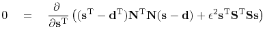
To review basic concepts, suppose we are in the one-dimensional frequency domain. Then the solution to the fitting goals (10) and (9) amounts to minimizing a quadratic form by setting to zero its derivative, say
 |
(11) |
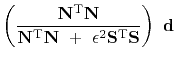
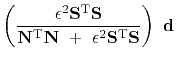
The analytic solutions in equations (12) and (13) are valid in 2-D Fourier space or dip space too. I prefer to compute them in the time and space domain to give me tighter control on window boundaries, but the Fourier solutions give insight and offer a computational speed advantage.
Let us express the fitting goal in the form needed in computation.
void signoi_lop (bool adj, bool add, int n1, int n2,
		 float *data, float *sign)
/*< linear operator >*/
{
    sf_helicon_init (nn);
    sf_polydiv_init (nd, ss);

    sf_adjnull(adj,add,n1,n2,data,sign);

    sf_helicon_lop (false, false, n1, n1, data, dd);
    sf_solver_prec(sf_helicon_lop, sf_cgstep, sf_polydiv_lop,
		   nd, nd, nd, sign, dd, niter, eps,
		   "verb", verb, "end");
    sf_cgstep_close();

    nn++;
    ss++;
}
|
|
|
|
|
Nonstationarity: patching |
![$\displaystyle \left[ \begin{array}{c} \bold 0 \\ \bold 0 \end{array} \right] \q...
... s \ +\ \left[ \begin{array}{c} -\bold N \bold d \\ \bold 0 \end{array} \right]$](img58.png)