Computational part 1

In the first part of the computational assignment, you will investigate the numerical accuracy of a finite-difference eikonal solver.

from rsf.proj import *
from rsf.prog import RSFROOT
import math

# Program compilation
#####################

proj = Project()

# COMMENT THE NEXT LINE FOR FORTRAN OR PYTHON
prog = proj.Program('analytical.c')

# UNCOMMENT BELOW IF YOU WANT TO USE FORTRAN
#prog = proj.Program('analytical.f90',
#                   F90PATH=os.path.join(RSFROOT,'include'),
#                   LIBS=['rsff90']+proj.get('LIBS'))


# UNCOMMENT BELOW IF YOU WANT TO USE PYTHON
# prog = proj.Command('analytical.exe','analytical.py',
#                    'cp $SOURCE $TARGET')
#AddPostAction(prog,Chmod(prog,0o755))

exe = str(prog[0])

# Velocity model
########################################
v0 = 0.5        # velocity at the origin
gz = 0.8        # vertical gradient
gx = 0.6        # horizontal gradient
nz = 601        # depth samples
nx = 1201       # lateral samples
dz = 0.5/(nz-1) # depth sampling
dx = 1.0/(nx-1) # lateral sampling

# v(z,x) = v0*/sqrt(1 - 2*v0*v0*(gz*z + gx*x))
##############################################

# !!! COMMENT BELOW !!!

Flow('vel',None,
       '''
       math n1=%d d1=%g n2=%d d2=%g
       output="%g/sqrt(1-%g*(%g*x1+%g*x2))"
       ''' % (nz,dz,nx,dx,v0,2*v0*v0,gz,gx))

# v(z,x) = v0 + gz*z + gx*x
###########################

# !!! UNCOMMENT BELOW !!!

#Flow('vel',None,
#      '''
#      math n1=%d d1=%g n2=%d d2=%g
#      output="%g+%g*x1+%g*x2"
#      ''' % (nz,dz,nx,dx,v0,gz,gx))

Plot('vel',
     '''
     grey color=j allpos=y screenht=6 screenratio=%g
     bias=%g wanttitle=n barreverse=y
     label1=Depth unit1=km label2=Lateral unit2=km
     scalebar=y barlabel=Velocity barunit="km/s" 
     ''' % ((nz-1.)/(nx-1.),v0))

# Analytical traveltime
########################

# !!! CHANGE case=s to case=v BELOW !!!

Flow('time',['vel',exe],
     '''
     ./${SOURCES[1]} v0=%g g1=%g g2=%g case=s
     ''' % (1./(v0*v0),-gz,-gx))
Plot('time',
     '''
     contour scalebar=y plotcol=7 c0=0 dc=0.1 nc=30
     screenht=6 screenratio=%g plotfat=5 wanttitle=n
     ''' % ((nz-1.)/(nx-1.)))

# Plot wavefronts overlayed on the velocity model
#################################################
Result('exact','vel time','Overlay')

errs = []
spaces = []

for sample in range(1,nz//30):

    # Subsample velocity and analytical traveltime
    ##############################################
    vel = 'vel%d' % sample
    tim = 'tim%d' % sample
    window = 'window j1=%d j2=%d' % (sample,sample)
    
    Flow(vel,'vel',window)
    Flow(tim,'time',window)

    space = 'spc%d' % sample
    h = sample*math.hypot(dx,dz)
    Flow(space,None,'spike n1=1 mag=%g' % h)
    spaces.append(space)

    # Solve the eikonal equation
    ############################
    eik = 'eik%d' % sample

    # !!!!!!!!! CHANGE BELOW !!!!!!!!!!
    
    Flow(eik,vel,
         '''
         eikonal yshot=0 order=1 br1=%g br2=%g
         ''' % (20*dz,20*dx))

    # Compute error
    ###############
    err = 'err%d' % sample
    Flow(err,[eik,tim],
         '''
         math ref=${SOURCES[1]} output="abs(input-ref)" |
         stack axis=2 norm=y | stack axis=1 norm=y 
         ''')
    errs.append(err)

# Concatenate results
#####################
cat = 'cat axis=1 ${SOURCES[1:%d]}' % len(spaces)
   
Flow('space',spaces,cat)
Flow('logspace','space','math output="log(input)" ')

Flow('err',errs,cat)
Flow('logerr','err','math output="log(input)" ')

graph = 'cmplx ${SOURCES[0:2]} | graph wanttitle=n '
for case in ('0','1'):
    Plot('err'+case,'space err',graph + '''
    label1="Grid Spacing" unit1=km
    label2=Error unit2=s
    ''',stdin=0)
    Plot('logerr'+case,'logspace logerr',graph + '''
    label1="Log(Grid Spacing)" unit1=
    label2="Log(Error)" unit2= grid=y
    ''',stdin=0)
    graph = graph + 'symbol=x plotcol=2 '

# Plot error versus spacing
###########################
Plot('err','err0 err1','Overlay')

# Plot error versus spacing on a logarithmic scale
##################################################
Plot('logerr','logerr0 logerr1','Overlay')

Result('err','err logerr','SideBySideAniso')

End()

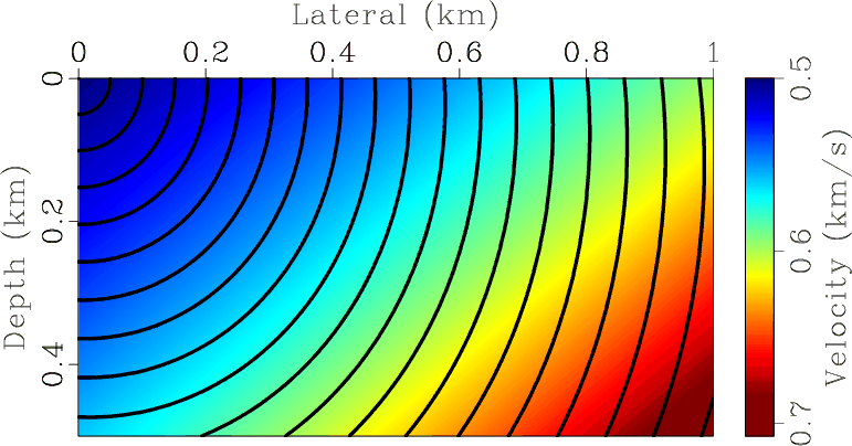
Figure 1 shows wavefronts in a medium with a constant gradient of slowness squared computed with an analytical two-point ray tracing formula from the class.


exact Figure 1. Wavefronts in a constant velocity gradient medium computed with an analytical formula.

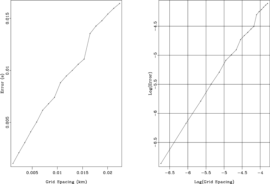
By computing traveltimes numerically at different sampling intervals and comparing the numerical result with the analytical one, we can get an experimental estimate of the numerical error behavior. The error is shown in Figure 2. The right plot in Figure 2 displays the error in logarithmic coordinates. The slope of the line in these coordinates shows directly the rate of convergence of the numerical method. For example, a first-order accurate method should have a slope of one.


err Figure 2. Left: average error of the finite-difference eikonal solver as a function of grid spacing. Right: the same on a log-log plot. The slope of the curve on the log-log plot indicates the order of the numerical accuracy.