Conjugate guided gradient (CGG) method for robust inversion and its application to velocity-stack inversion

CG method for LS Inversion

Most inversion problems start by formulating the forward problem, which describes the forward operator $\mathbf L$ that transforms the model vector $\mathbf m$ into the data vector $\mathbf d$

$$\mathbf d = \mathbf L \mathbf m .$$ (1)

In general, the measured data $\mathbf d$ may be inexact, and the forward operator $\mathbf L$ may be ill-conditioned. In that case, instead of solving the above equation directly, different approaches are used to find an optimum solution $\mathbf m$ for given data $\mathbf d$. The most popular method is finding a solution that minimizes the misfit between the data $\mathbf d$ and the modeled data $\mathbf L\mathbf m$. The misfit is often referred as residual vector $\mathbf r$ and is described as follows:

$$\mathbf r = \mathbf L\mathbf m - \mathbf d .$$ (2)

In least-squares inversion, the solution $\mathbf m$ is the one that minimizes the squares of the residual vector as follows:

$$min_m ({\mathbf r^T r}) = min_m {(\mathbf L\mathbf m - \mathbf d)^T(\mathbf L\mathbf m - \mathbf d)} .$$ (3)

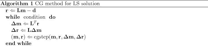
Most iterative solvers for the LS problem search the minimum solution on a line or a plane in the solution space. In the CG algorithm, not a line, but rather a plane is searched. A plane is made from an arbitrary linear combination of two vectors. One vector is chosen to be the gradient vector. The other vector is chosen to be the previous descent step vector. Following Claerbout (1992), a conjugate-gradient algorithm for the LS solution can be summarized as shown in Algorithm 1.

In Algorithm 1, the $\rm condition$ represents a convergence check such as the tolerance of residual vector $\mathbf r$, a maximum number of iteration, and so on. The subroutine cgstep() updates model $\mathbf m$ and residual $\mathbf r$ using the previous iteration descent vector in the conjugate space $\Delta \mathbf s = L (\mathbf m_i - \mathbf m_{i-1})$, where $i$ is the iteration step, and the conjugate gradient vector $\Delta \mathbf r$. The update step size is determined by minimizing the quadrature function composed from $\Delta \mathbf r$ (the conjugate gradient) and $\Delta \mathbf s$ (the previous iteration descent vector in the conjugate space) as follows Claerbout (1992):

$$Q(\alpha,\beta) = (\mathbf r-\alpha \Delta \mathbf r -\beta \... ... (\mathbf r-\alpha \Delta \mathbf r -\beta \Delta \mathbf s) .$$

Notice that the gradient vector ( $\Delta \mathbf m$) in the CG method for LS solution is the gradient of the squared residual and is determined by taking the derivative of the squared residual (i.e. the $\ell^2$-norm of the residual, $\mathbf r^T \mathbf r$) with respect to the model $\mathbf m^T$:

$$\Delta \mathbf m = {\partial \over \partial \mathbf m^T } (... ...f d)^T(\mathbf L\mathbf m -\mathbf d) = \mathbf L^T\mathbf r .$$ (4)

Conjugate guided gradient (CGG) method for robust inversion and its application to velocity-stack inversion