Adaptive prediction filtering in $t$ -$x$ -$y$ domain for random noise attenuation using regularized nonstationary autoregression

$t$ -$x$ adaptive prediction filtering using RNA

Consider a 2D prediction filter (general for stationary PF) with ten prediction coefficients $B_{i,j}$ :

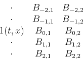$$\begin{array}{ccc} \cdot &B_{-2,1} &B_{-2,2} \ \cdot &B_{-1,... ... \cdot &B_{1,1} &B_{1,2} \ \cdot &B_{2,1} &B_{2,2} \end{array}$$ (1)

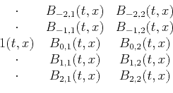
where $i$ is time shift, $j$ is space shift, the vertical axis is time axis, and the horizontal axis is space axis. The output position is under the ``$1(t,x)$ '' coefficient on the left side of filter and ``$1(t,x)$ '' indicates time- and space-varying samples. The filter is noncausal along the time axis and causal along the space axis. More filter structures will be discussed later. The PF has the different coefficients from PEF, which includes causal time prediction coefficients.

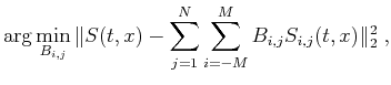
To obtain stationary PF coefficients, one can solve the over-determined least-squares problem 2pt

$$\tilde{B}_{i,j} = \arg\min_{B_{i,j}}\Vert S(t,x)- \sum_{j=1}^{N}\sum_{i=-M}^{M} B_{i,j}S_{i,j}(t,x)\Vert _2^2 \;,$$ (2)

where $S_{i,j}(t,x)$ represents the translation of linear events $S(t,x)$ in both time and space directions with time shift $i$ and space shift $j$ . The choice of the filter size depends on the maximum dip of the plane waves in the data and the number of dips. For nonlinear events, cutting data into overlapping windows (patching) is a common method to handle nonstationarity (Claerbout, 2010), although it occasionally fails in the presence of variable dips.

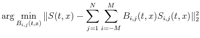
For nonstationary situations, we can also assume local linearization of the data. For estimating APF coefficients, nonstationary autoregression allows the coefficients $B_{i,j}$ to change with both $t$ and $x$ . The new adaptive filter can be designed as

$$\begin{array}{ccc} \cdot &B_{-2,1}(t,x) &B_{-2,2}(t,x) \ \cd... ... &B_{1,2}(t,x) \ \cdot &B_{2,1}(t,x) &B_{2,2}(t,x) \end{array}$$ (3)

In the linear notation, prediction coefficients $B_{i,j}(t,x)$ can be obtained by solving the under-determined least-squares problem 2pt

$$\tilde{B}_{i,j}(t,x) = \arg\min_{B_{i,j}(t,x)}\Vert S(t,x)- \sum_{j=1}^{N} \sum_{i=-M}^{M} B_{i,j}(t,x)S_{i,j}(t,x)\Vert _2^2$$

$$+ \epsilon^2 \sum_{j=1}^{N} \sum_{i=-M}^{M} \Vert\mathbf{D}[B_{i,j}(t,x)]\Vert _2^2\;,$$ (4)

where $\mathbf{D}$ is the regularization operator and $\epsilon$ is a scalar regularization parameter. This approach was described by Fomel (2009) as regularized nonstationary autoregression (RNA). Shaping regularization (Fomel, 2007) specified a shaping (smoothing) operator $\mathbf{R}$ instead of $\mathbf{D}$ and provided better numerical properties than Tikhonov's regularization (Tikhonov, 1963) in equation 4. The advantages of the shaping regularization include an intuitive selection of regularization parameters and fast iteration convergence. Coefficients $B_{i,j}(t,x)$ get constrained by regularization. The required parameters are the size and shape of the filter, $B_{i,j}(t,x)$ , and the smoothing radius for shaping regularization. The size of APF controls the range and the number of the predicted dips. Larger filter parameters, $N$ and $M$ , are able to predict more accurate dips, however, the APFs with the large filter size pass more random noise and add more computational cost. As the smoothing radius of the APF increases, the APF removes not only more random noise but also some structural details. The APF is able to be extended to the adaptive PEF (APEF), which shows a expected representation of nonstationary signal and is fit for seismic data interpolation (Liu and Fomel, 2011) and random noise attenuation (Liu and Liu, 2011). However, the structure of APEF is different from that of APF, which excludes the causal time prediction coefficients and forces only lateral predictions. Meanwhile, in this paper, we use a two-step method that estimates APF coefficients by solving an under-determined problem and calculates noise-free signal. The proposed method is different from the two-step APEF denoising including APEF estimation for signal and noise plus signal and noise separation by solving a least-square system as shown in Liu and Liu (2011).

Adaptive prediction filtering in $t$ -$x$ -$y$ domain for random noise attenuation using regularized nonstationary autoregression