|
|
|
|
Local seismic attributes |
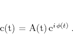
Let ![]() represent seismic trace as a function of time
represent seismic trace as a function of time ![]() . The
corresponding complex trace
. The
corresponding complex trace ![]() is defined as
is defined as
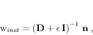
Note that the definition of instantaneous frequency calls for division
of two signals. In a linear algebra notation,
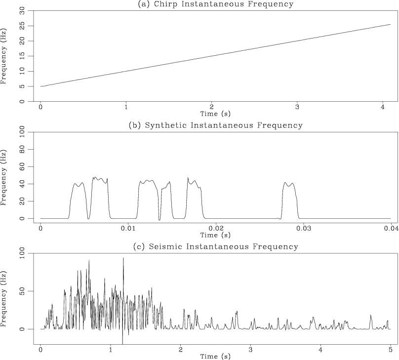
Figure ![]() shows three test signals for comparing frequency
attributes. The first signal is a synthetic chirp function with
linearly varying frequency. Instantaneous frequency shown in
Figure 1 correctly estimates the modeled frequency trend.
The second signal is a piece of a synthetic seismic trace obtained by
convolving a 40-Hz Ricker wavelet with synthetic reflectivity. The
instantaneous frequency (Figure 1b) shows many variations
and appears to contain detailed information. However, this information
is useless for characterizing the dominant frequency content of the
data, which remains unchanged due to stationarity of the seismic
wavelet. The last test example (Figure
shows three test signals for comparing frequency
attributes. The first signal is a synthetic chirp function with
linearly varying frequency. Instantaneous frequency shown in
Figure 1 correctly estimates the modeled frequency trend.
The second signal is a piece of a synthetic seismic trace obtained by
convolving a 40-Hz Ricker wavelet with synthetic reflectivity. The
instantaneous frequency (Figure 1b) shows many variations
and appears to contain detailed information. However, this information
is useless for characterizing the dominant frequency content of the
data, which remains unchanged due to stationarity of the seismic
wavelet. The last test example (Figure ![]() c) is a real
trace extracted from a seismic image. The instantaneous frequency
(Figure 1c) appears noisy and even contains physically
unreasonable negative values. Similar behavior was described by
White (1991).
c) is a real
trace extracted from a seismic image. The instantaneous frequency
(Figure 1c) appears noisy and even contains physically
unreasonable negative values. Similar behavior was described by
White (1991).
|
|---|
|
inst
Figure 1. Instantaneous frequency of test signals from Figure |
|
|
|
|---|
|
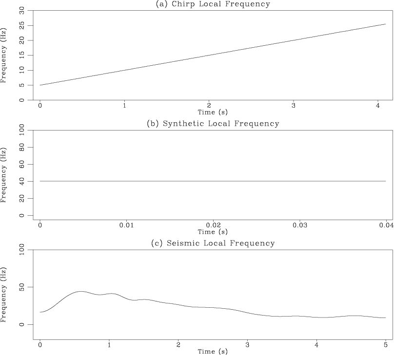
locl
Figure 2. Local frequency of test signals from Figure |
|
|
|
|
|
|
Local seismic attributes |
![\begin{displaymath}
\omega(t) = \phi'(t) = \mathit{Im}\left[\frac{c'(t)}{c(t)}\right]
= \frac{f(t)\,h'(t) - f'(t)\,h(t)}{f^2(t) + h^2(t)}\;.
\end{displaymath}](img9.png)