Local seismic attributes

Definition of local correlation

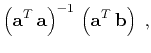
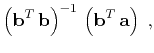
In a linear algebra notation, the squared correlation coefficient $\gamma$ from equation 8 can be represented as a product of two least-squares inverses

$$\gamma^2 = \gamma_1\,\gamma_2\;,$$ (9)

$$\gamma_1 = \left(\mathbf{a}^T\,\mathbf{a}\right)^{-1}\,\left(\mathbf{a}^T\,\mathbf{b}\right)\;,$$ (10)

$$\gamma_2 = \left(\mathbf{b}^T\,\mathbf{b}\right)^{-1}\,\left(\mathbf{b}^T\,\mathbf{a}\right)\;,$$ (11)

where $\mathbf{a}$ is a vector notation for $a(t)$, $\mathbf{b}$ is a vector notation for $b(t)$, and $\mathbf{x}^T\,\mathbf{y}$ denotes the dot product operation. Let $\mathbf{A}$ be a diagonal operator composed from the elements of $\mathbf{a}$ and $\mathbf{B}$ be a diagonal operator composed from the elements of $\mathbf{b}$. Localizing equations 10-11 amounts to adding regularization to inversion. Scalars $\gamma_1$ and $\gamma_2$ turn into vectors $\mathbf{c}_1$ and $\mathbf{c}_2$ defined, using shaping regularization , as

$$\mathbf{c}_1 = \left[\lambda^2\,\mathbf{I} + \mathbf{S}\,\left(\mathbf{A}^T\,\ma... ...mbda^2\,\mathbf{I}\right)\right]^{-1}\, \mathbf{S}\,\mathbf{A}^T\,\mathbf{b}\;,$$ (12)

$$\mathbf{c}_2 = \left[\lambda^2\,\mathbf{I} + \mathbf{S}\,\left(\mathbf{B}^T\,\ma... ...mbda^2\,\mathbf{I}\right)\right]^{-1}\, \mathbf{S}\,\mathbf{B}^T\,\mathbf{a}\;.$$ (13)

To define a local similarity measure, I apply the component-wise product of vectors $\mathbf{c}_1$ and $\mathbf{c}_2$. It is interesting to note that, if one applies an iterative conjugate-gradient inversion for computing the inverse operators in equations 12 and 13, the output of the first iteration will be the smoothed product of the two signals $\mathbf{c}_1 = \mathbf{c}_2 = \mathbf{S}\,\mathbf{A}^T\,\mathbf{b}$, which is equivalent, with an appropriate choice of $\mathbf{S}$, to the algorithm of fast local cross-correlation proposed by Hale (2006).

The local similarity attribute is useful for solving the problem of multicomponent image registration. After an initial registration using interpreter's ``nails'' (DeAngelo et al., 2004) or velocities from seismic processing, a useful registration indicator is obtained by squeezing and stretching the warped shear-wave image while measuring its local similarity to the compressional image. Such a technique was named residual $\gamma$ scan and proposed by Fomel et al. (2005). Figure 6 shows a residual scan for registration of multicomponent images from Figure 4. Identifying and picking points of high local similarity enables multicomponent registration with high-resolution accuracy. The registration result is visualized in Figure 7, which shows interleaved traces from PP and SS images before and after registration. The alignment of main seismic events is an indication of successful registration.

vec-sc-0
Figure 6. Residual warping scan for multicomponent PP/SS registration computed with the help of the local similarity attribute. Picking maximum similarity trends enables multicomponent registration.

vec-in0-0,vec-in1-1
Figure 7. Interleaved traces from PP and warped SS images before (a) and after (b) multicomponent registration. The checkerboard pattern on major seismic events in (a) disappears in (b) which is an indication of successful registration.

Local seismic attributes