 |
 |
 |
 | Exploring three-dimensional implicit wavefield extrapolation
with the helix transform |  |
![[pdf]](icons/pdf.png) |
Next: Helix and multidimensional deconvolution
Up: Spectral factorization and three-dimensional
Previous: Spectral factorization and three-dimensional
The conventional way of applying implicit finite-difference schemes
reduces to solving a system of linear equations with a sparse matrix.
For example, to apply the scheme of equation (11), we
can put the filter denominator on the other side of the extrapolation
equation, writing it as
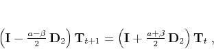 |
(14) |
where  is the identity matrix,
  is the convolution
matrix for filter (10), and
is the convolution
matrix for filter (10), and  is the vector of
temperature distribution at time level
is the vector of
temperature distribution at time level  . In the case of
two-dimensional extrapolation, the matrix on the left side of equation
(14) takes the tridiagonal form
. In the case of
two-dimensional extrapolation, the matrix on the left side of equation
(14) takes the tridiagonal form
![\begin{displaymath}
\mathbf{A} = \left(\mathbf{I} -c\,\mathbf{D}_2\right) =
\l...
...n-1} \\
0 & & & & -c_{n} & 1 + 2c_{n}
\end{array}\right]\;,
\end{displaymath}](img48.png) |
(15) |
where
 , and where, for simplicity, we assume
zero-slope boundary conditions. Like any positive-definite tridiagonal
matrix, matrix
, and where, for simplicity, we assume
zero-slope boundary conditions. Like any positive-definite tridiagonal
matrix, matrix  can be inverted recursively by an
  decomposition into two bidiagonal matrices. The cost of inversion is
directly proportional to the number of vector components. The same
conclusion holds for the case of depth extrapolation [equation
(13)] with the substitution
decomposition into two bidiagonal matrices. The cost of inversion is
directly proportional to the number of vector components. The same
conclusion holds for the case of depth extrapolation [equation
(13)] with the substitution
 .
.
In the case of a laterally constant coefficient  , we can take a
different point of view on the tridiagonal matrix inversion. In this
case, the matrix
, we can take a
different point of view on the tridiagonal matrix inversion. In this
case, the matrix  represents a convolution with a
symmetric three-point filter
represents a convolution with a
symmetric three-point filter  . The
decomposition of such a matrix is precisely equivalent to filter
factorization into the product of a causal minimum-phase filter
with its adjoint. This conclusion can be confirmed by the easily
verified equality
. The
decomposition of such a matrix is precisely equivalent to filter
factorization into the product of a causal minimum-phase filter
with its adjoint. This conclusion can be confirmed by the easily
verified equality
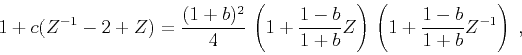 |
(16) |
where
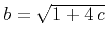 . The inverse of the causal minimum-phase
filter
. The inverse of the causal minimum-phase
filter
 is a recursive inverse filter.
Correspondingly, the inverse of its adjoint pair,
is a recursive inverse filter.
Correspondingly, the inverse of its adjoint pair,
 , is the same inverse filtering, performed in the adjoint mode
(backwards in space). In the next subsection, we show how this
approach can be carried into three dimensions by applying the helix
transform.
, is the same inverse filtering, performed in the adjoint mode
(backwards in space). In the next subsection, we show how this
approach can be carried into three dimensions by applying the helix
transform.
|
|
|
|
| Exploring three-dimensional implicit wavefield extrapolation
with the helix transform | |
|
Next: Helix and multidimensional deconvolution
Up: Spectral factorization and three-dimensional
Previous: Spectral factorization and three-dimensional
2014-02-17