Huygens wavefront tracing: A robust alternative to conventional ray tracing

The Marmousi model

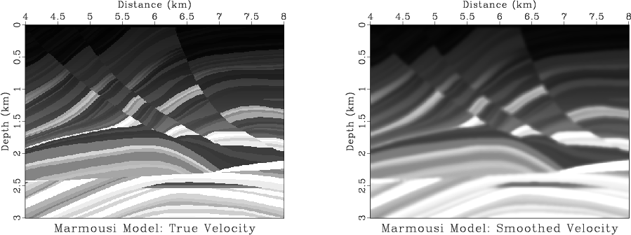
In the third example, we have applied the same method to trace rays in the far more complex Marmousi 2-D Model. Figure 11 contains the true velocity (left) and a smoothed version using twice a tridiagonal $5\times5$ filter (right). In Figure 12 we present the rays obtained on the unsmoothed Marmousi Model with the PRT method (left) and with the HWT method (right). In Figure 13 we present the rays obtained on the smoothed Marmousi Model with the PRT method (left) and with the HWT method (right).

m-velocity
Figure 11. The Marmousi model. The true velocity appears on the left,the smoothed velocity on the right.

m-velrw-raw
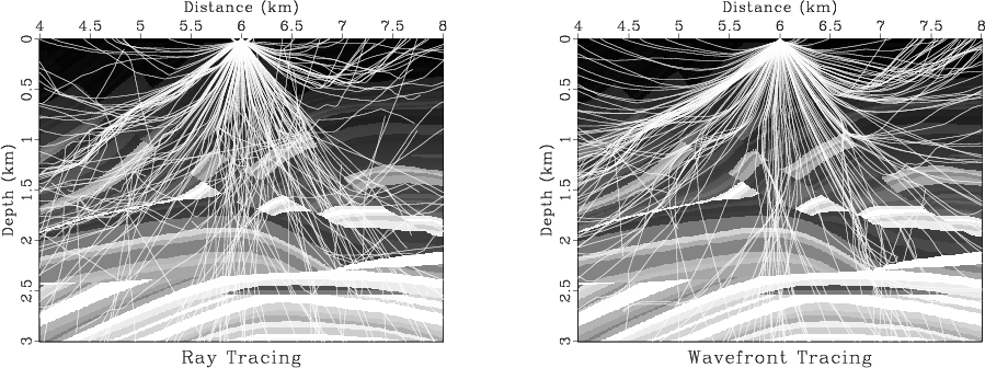
Figure 12. The rays obtained in the true velocity Marmousi model using the PRT method (left) and the HWT method (right).

m-velrw-smooth
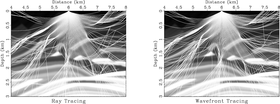
Figure 13. The rays obtained in the smoothed Marmousi model using the PRT method (left) and the HWT method (right).

As expected, the rays traced using the PRT method (Figure 12, left), which represents a more exact solution to the eikonal equation for the given velocity field, have a very rough distribution. Since this erratic result is of no use in practice, regardless of its accuracy, the only way to get a proper result is to apply the ray tracing to a smoothed velocity model (Figure 13, left).

On the other hand, the result obtained with the HWT method looks a lot better, though some imperfections are still visible. For the case of the unsmoothed velocity medium, the rays have a much smoother pattern, which is less dependent on how rough the velocity model is (Figure 12, right). This feature is preserved in the case of the smoothed model (Figure 13, right) where the distributions of rays displayed by the two methods are much more similar, though some differences remain (see, for example the zone around x=6.5km, z=2.0km).

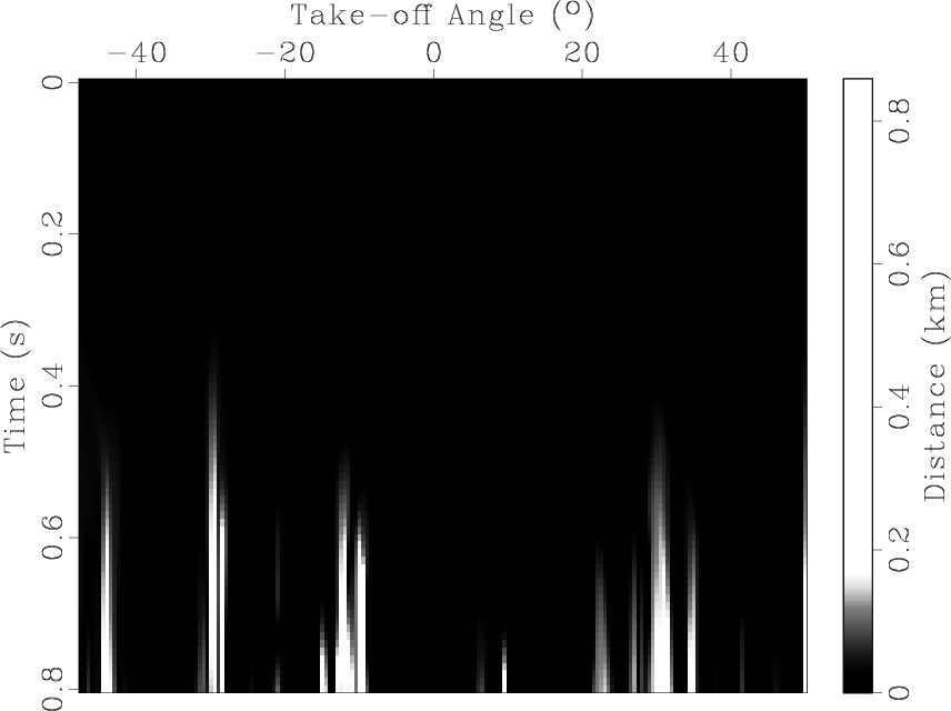
As with the Gaussian model, we present the distances between the points that correspond to the same ray, identified by the same take-off angle, at the same traveltimes (Figure 14). This is another way to interpret what we saw in Figure 13, where most of the rays have a consistent behavior, displaying similar paths regardless of the method used, and therefore small distances, and a few have a different trajectory, resulting in big distances that increase with traveltime.

m-diff-smooth Figure 14. The distance between the corresponding points on the rays obtained with the PRT method and with the HWT method. Distances are given in meters.

Huygens wavefront tracing: A robust alternative to conventional ray tracing