Multidimensional recursive filter preconditioning in geophysical estimation problems

Data-space regularization (model preconditioning)

The data-space regularization approach is closely connected with the concept of model preconditioning. We can introduce a new model $\mathbf{p}$ with the equality

$$\mathbf{m = P p}\;,$$ (8)

where $\mathbf {P}$ is a preconditioning operator. The residual vector $\mathbf{r}$ for the data-fitting goal (1) can be defined by the relationship

$$\epsilon \mathbf{r = d - L m = d - L P p}\;,$$ (9)

where $\epsilon$ is the same scaling parameter as in (2) - the reason for this choice will be clear from the analysis that follows. Let us consider a compound model $\hat{\mathbf{p}}$, composed of the preconditioned model vector $\mathbf{p}$ and the residual $\mathbf{r}$:

$$\hat{\mathbf{p}} = \left[\begin{array}{c} \mathbf{p} \mathbf{r} \end{array}\right]\;.$$ (10)

With respect to the compound model, we can rewrite equation (9) as

$$\left[\begin{array}{cc} \mathbf{L P} & \epsilon \mathbf{I} ... ...array}\right] = \mathbf{G_d} \hat{\mathbf{p}} = \mathbf{d}\;,$$ (11)

where $\mathbf{G_d}$ is a row operator:

$$\mathbf{G_d} = \left[\begin{array}{cc} \mathbf{L P} & \epsilon \mathbf{I} \end{array}\right]\;,$$ (12)

and $\mathbf{I}$ represents the data-space identity operator.

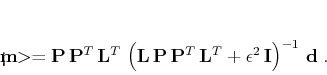
Equation (11) is clearly underdetermined with respect to the compound model $\hat{\mathbf{p}}$. If from all possible solutions of this system we seek the one with the minimal power $\hat{\mathbf{p}}^T \hat{\mathbf{p}}$, the formal result takes the well-known form

$$<\!\!\hat{\mathbf{p}}\!\!> = \left[\begin{array}{c} <\!\!\m... ...lon^2 \mathbf{I}\right)^{-1} \mathbf{d} \end{array} \right]\;.$$ (13)

Applying equation (8), we obtain the corresponding estimate $<\!\!\mathbf{m}\!\!>$ for the initial model $\mathbf{m}$, as follows:

$$<\!\!\mathbf{m}\!\!> = \mathbf{P} \mathbf{P}^T \mathbf{... ...hbf{L}^T + \epsilon^2 \mathbf{I}\right)^{-1} \mathbf{d}\;.$$ (14)

It is easy to show algebraically that estimate (14) is equivalent to estimate (7) under the condition

$$\mathbf{C} = \mathbf{P} \mathbf{P}^T = \left(\mathbf{D}^T \mathbf{D}\right)^{-1}\;,$$ (15)

where we need to assume the self-adjoint operator $\mathbf{D}^T \mathbf{D}$ to be invertible.

To prove the equivalence, consider the operator

$$\mathbf{G} = \mathbf{L}^T \mathbf{L} \mathbf{C} \mathbf{L}^T + \epsilon^2 \mathbf{L}^T\;,$$ (16)

which is a mapping from the data space to the model space. Grouping the multiplicative factors in two different ways, we can obtain the equality

$$\mathbf{G} = \mathbf{L}^T \left(\mathbf{L} \mathbf{C} \ma... ...\epsilon^2 \mathbf{C}^{-1}\right) \mathbf{C} \mathbf{L}^T\;,$$ (17)

or, in another form,

$$\mathbf{C} \mathbf{L}^T \left(\mathbf{L} \mathbf{C} \mat... ...L} + \epsilon^2 \mathbf{C}^{-1}\right)^{-1} \mathbf{L}^T\;.$$ (18)

The left-hand side of equality (18) is exactly the projection operator from formula (14), and the right-hand side is the operator from formula (7).

This proves the legitimacy of the alternative data-space approach to data regularization: the model estimation is reduced to a least-squares minimization of the specially constructed compound model $\hat{\mathbf{p}}$ under the constraint (9).

We summarize the differences between the model-space and data-space regularization in Table 1.

	Model-space	Data-space
effective model	$\mathbf{m}$	$\hat{\mathbf{p}} = \left[\begin{array}{c} \mathbf{p} \mathbf{r} \end{array}\right]$
effective data	$\hat{\mathbf{d}} = \left[\begin{array}{c} \mathbf{d} \mathbf{0} \end{array}\right]$	$\mathbf{d}$
effective operator	$\mathbf{G_m} = \left[\begin{array}{c} \mathbf{L} \\ \epsilon \mathbf{D} \end{array}\right]$	$\mathbf{G_d} = \left[\begin{array}{cc} \mathbf{LP} & \epsilon \mathbf{I} \end{array}\right]$
optimization problem	minimize $\hat{\mathbf{r}}^T \hat{\mathbf{r}}$, where $\hat{\mathbf{r}} = \hat{\mathbf{d}} - \mathbf{G_m m}$	minimize $\hat{\mathbf{p}}^T \hat{\mathbf{p}}$ under the constraint $\mathbf{G_d} \hat{\mathbf{p}} = \mathbf{d}$
formal estimate for $\mathbf{m}$	$\left(\mathbf{L}^T \mathbf{L} + \epsilon^2 \mathbf{C}^{-1}\right) \mathbf{L}^T \mathbf{d}$, where $\mathbf{C}^{-1} = \mathbf{D}^T \mathbf{D}$	$\mathbf{C L}^T (\mathbf{L C L}^T + \epsilon^2 \mathbf{I})^{-1} \mathbf{d}$, where $\mathbf{C} = \mathbf{P P}^T$.

Table 1. Comparison between model-space and data-space regularization

Although the two approaches lead to similar theoretical results, they behave quite differently in the process of iterative optimization. In the next section, we illustrate this fact with many examples and show that in the case of incomplete optimization, the second (preconditioning) approach is generally preferable.

Multidimensional recursive filter preconditioning in geophysical estimation problems