|
|
|
|
Asymptotic pseudounitary stacking operators |
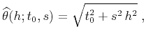
Velocity transform is another form of hyperbolic stacking with the summation path
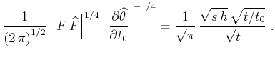
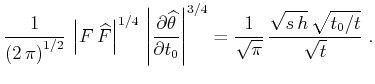
Solving equation (69) for ![]() , we find that the asymptotic
inverse and adjoint operators have the elliptic summation path
, we find that the asymptotic
inverse and adjoint operators have the elliptic summation path
| (70) |
Figure 4 shows the output of a numerical test of the least-squares velocity transform inversion using a CMP gather from the Mobil AVO dataset (Lumley et al., 1995). The input CMP gather (shown in the left plot of Figure 5) is inverted using an iterative conjugate-gradient method and two different weighting scheme: the uniform weighting and the asymptotic pseudo-unitary weights (71-72). Analogously to Figure 1, the iterative convergence is measured by the least-squares norm of the data residual error at different iterations. Figure 4 shows that the pseudo-unitary weighting provides a noticeably faster convergence at the first three iterations. At later iterations, the residual errors of the two methods are very close to each other. The use of a pseudo-unitary weighting will be justified in this case if only three iterations are practically affordable. The results of inversion after 10 conjugate-gradient iterations are plotted in Figures 5 and 6. The right plot in Figure 5 shows the output of the velocity transform inversion: an optimized velocity scan. Figure 6 shows the corresponding modeled CMP gather and the residual error. The error is negligible which indicates a successful inversion.
|
cgiter
Figure 4. Comparison of convergence of the iterative velocity transform inversion. The dashed line corresponds to the unweighted (uniformly weighted) operator. The solid line corresponds to the asymptotic pseudo-unitary operator. The latter provides a faster convergence at early iterations. |

|
|---|---|
|
|

|
|---|
|
dircvv
Figure 5. Input CMP gather (left) and its velocity transform counterpart (right) after 10 iterations of iterative least-squares inversion. |
|
|

|
|---|
|
dirrst
Figure 6. The modeled CMP gather (left) and the residual error (right) plotted at the same scale. |
|
|
|
|
|
|
Asymptotic pseudounitary stacking operators |