|
 |
 |
 | Velocity continuation and the anatomy of
residual prestack time migration |  |
![[pdf]](icons/pdf.png) |
Next: About this document ...
Up: Fomel: Velocity continuation
Previous: Acknowledgments
-
Adler, F., 2002, Kirchhoff image propagation: Geophysics, 67, 126-134.
-
-
Al-Yahya, K., and P. Fowler, 1986, Prestack residual migration, in
SEP-50: Stanford Exploration Project, 219-230.
-
-
Beasley, C., W. Lynn, K. Larner, and H. Nguyen, 1988, Cascaded
frequency-wavenumber migration - Removing the restrictions on depth-varying
velocity: Geophysics, 53, 881-893.
-
-
Belonosova, A. V., and A. S. Alekseev, 1967, in About one formulation of
the inverse kinematic problem of seismics for a two-dimensional continuously
heterogeneous medium: Nauka, 137-154.
-
-
Berkhout, A. J., 1985, Seismic migration: Imaging of acoustic energy by wave
field extrapolation: Elsevier, Amsterdam.
-
-
Chun, J. H., and C. A. Jacewitz, 1981, Fundamentals of frequency-domain
migration: Geophysics, 46, 717-733.
-
-
Claerbout, J. F., 1985, Imaging the Earth's Interior: Blackwell Scientific
Publications.
-
-
----, 1986, Velocity extrapolation by cascaded 15 degree migration, in SEP-48: Stanford Exploration Project, 79-84.
-
-
Clayton, R. W., 1978, Common midpoint migration, in SEP-14: Stanford
Exploration Project, 21-36.
-
-
Courant, R., and D. Hilbert, 1989, Methods of mathematical physics: John Wiley
& Sons.
-
-
Deregowski, S. M., 1990, Common-offset migrations and velocity analysis: First
Break, 08, 224-234.
-
-
Dunkin, J. W., and F. K. Levin, 1973, Effect of normal moveout on a seismic
pulse: Geophysics, 38, 635-642.
-
-
Etgen, J., 1990, Residual prestack migration and interval velocity estimation:
PhD thesis, Stanford University.
-
-
Fomel, S., 1997, Velocity continuation and the anatomy of prestack residual
migration: 67th Ann. Internat. Mtg, Soc. of Expl. Geophys., 1762-1765.
-
-
----, 2001, Migration velocity analysis by velocity continuation: 71st Ann.
Internat. Mtg, Soc. of Expl. Geophys., 1107-1110.
-
-
----, 2003a, Theory of differential offset continuation: Geophysics, in
press.
-
-
----, 2003b, Time migration velocity analysis by velocity continuation:
Geophysics, submitted for publication.
-
-
Fomel, S. B., 1994, Method of velocity continuation in the problem of temporal
seismic migration: Russian Geology and Geophysics, 35, 100-111.
-
-
Fowler, P., 1984, Velocity independent imaging of seismic reflectors: 54th
Ann. Internat. Mtg, Soc. of Expl. Geophys., Session:S1.8.
-
-
----, 1988, Seismic velocity estimation using prestack time migration: PhD
thesis, Stanford University.
-
-
Gradshtein, I. S., and I. M. Ryzhik, 1994, Table of integrals, series, and
products: Boston: Academic Press.
-
-
Hale, I. D., 1983, Dip moveout by Fourier transform: PhD thesis, Stanford
University.
-
-
Hubral, P., M. Tygel, and J. Schleicher, 1996, Seismic image waves:
Geophysical Journal International, 125, 431-442.
-
-
Jakubowicz, H., and S. Levin, 1983, A simple exact method of three-dimensional
migration - Theory: Geophys. Prosp., 31, 34-56.
- (Discussion in GPR-34-06-0927-0939 with reply by author; Comment in
GPR-32-02-0347-0350 with reply by author).
-
Larner, K., and C. Beasley, 1987, Cascaded migrations - Improving the
accuracy of finite-difference migration: Geophysics, 52, 618-643.
- (Errata in GEO-52-8-1165).
-
Levin, S., 1986a, Cascaded fifteen degree equations simplified, in
SEP-48: Stanford Exploration Project, 101-108.
-
-
----, 1986b, Test your migration IQ, in SEP-48: Stanford
Exploration Project, 147-160.
-
-
Liptow, F., and P. Hubral, 1995, Migrating around in circles: The Leading
Edge, 14, 1125-1127.
-
-
Liu, H., and G. McMechan, 1996, Dynamic residual prestack depth migration for
common offset gathers: UTD Report.
-
-
Liu, Z., and N. Bleistein, 1995, Migration velocity analysis: Theory and an
iterative algorithm: Geophysics, 60, 142-153.
-
-
MacKay, S., and R. Abma, 1992, Imaging and velocity estimation with
depth-focusing analysis: Geophysics, 57, 1608-1622.
-
-
Mikulich, W., and D. Hale, 1992, Steep-dip v(z) imaging from an ensemble of
Stolt-like migrations: Geophysics, 57, 51-59.
-
-
Popovici, A. M., 1995, Prestack migration by split-step DSR, in
SEP-84: Stanford Exploration Project, 53-60.
-
-
Rothman, D. H., S. A. Levin, and F. Rocca, 1985, Residual migration -
Applications and limitations: Geophysics, 50, 110-126.
-
-
Sava, P., and S. Fomel, 2003, Wave-equation angle-domain common-image gathers:
Geophysics, in press.
-
-
Schleicher, J., P. Hubral, G. Hocht, and F. Liptow, 1997, Seismic
constant-velocity remigration: Geophysics, 62, 589-597.
-
-
Schneider, W. A., 1978, Integral formulation for migration in two-dimensions
and three-dimensions: Geophysics, 43, 49-76.
-
-
Shurtleff, R. N., 1984, An F-K procedure for prestack migration and
migration velocity analysis, in Presented at the 46th Annual EAGE Mtg.,
London: EAGE.
-
-
Stolt, R. H., 1978, Migration by Fourier transform: Geophysics, 43,
23-48.
- (Discussion and reply in GEO-60-5-1583).
-
----, 1996, Short note - A prestack residual time migration operator:
Geophysics, 61, 605-607.
-
-
Tygel, M., J. Schleicher, and P. Hubral, 1994, Pulse distortion in depth
migration: Geophysics, 59, 1561-1569.
-
-
Yilmaz, O., 1979, Prestack partial migration: PhD thesis, Stanford University.
-
-
Yilmaz, O., and R. E. Chambers, 1984, Migration velocity analysis by
wave-field extrapolation: Geophysics, 49, 1664-1674.
-
-
Yilmaz, O., and J. F. Claerbout, 1980, Prestack partial migration: Geophysics,
45, 1753-1779.
-
Appendix
A
DERIVING THE KINEMATIC EQUATIONS
The main goal of this appendix is to derive the partial differential
equation describing the image surface in a
depth-midpoint-offset-velocity space.
vlcray
Figure A-1. Reflection rays in a constant
velocity medium (a scheme).
|

|
![[png]](icons/viewmag.png) ![[xfig]](icons/xfig.png)
|
|---|
The derivation starts with observing a simple geometry of reflection
in a constant-velocity medium, shown in Figure A-1. The
well-known equations for the apparent slowness
 |
(52) |
 |
(53) |
relate the first-order traveltime derivatives for the reflected waves
to the emergence angles of the incident and reflected rays. Here  stands for the source location at the surface,
  is the receiver
location,
is the receiver
location,  is the reflection traveltime,
  is the constant
velocity, and
is the constant
velocity, and  and
and  are the angles shown in Figure
A-1. Considering the traveltime derivative with respect to
the depth of the observation surface
are the angles shown in Figure
A-1. Considering the traveltime derivative with respect to
the depth of the observation surface  shows that the
contributions of the two branches of the reflected ray, added
together, form the equation
shows that the
contributions of the two branches of the reflected ray, added
together, form the equation
 |
(54) |
It is worth mentioning that the elimination of angles from equations
(A-1), (A-2), and (A-3) leads to
the famous double-square-root equation,
 |
(55) |
published in the Russian literature by Belonosova and Alekseev (1967) and commonly
used in the form of a pseudo-differential dispersion relation
(Claerbout, 1985; Clayton, 1978) for prestack
migration (Popovici, 1995; Yilmaz, 1979). Considered
locally, equation (A-4) is independent of the constant velocity
assumption and enables recursive prestack downward
continuation of reflected waves in heterogeneous isotropic
media.
Introducing the midpoint coordinate
 and half-offset
 , one can apply the chain rule and elementary
trigonometric equalities to formulas (A-1) and
(A-2) and transform these formulas to
, one can apply the chain rule and elementary
trigonometric equalities to formulas (A-1) and
(A-2) and transform these formulas to
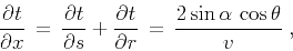 |
(56) |
 |
(57) |
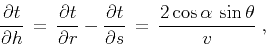
where
 is the dip angle, and
 is the reflection angle
(Claerbout, 1985; Clayton, 1978). Equation
(A-3) transforms analogously to
is the reflection angle
(Claerbout, 1985; Clayton, 1978). Equation
(A-3) transforms analogously to
 |
(58) |
This form of equation (A-3) is used to describe the stretching
factor of the waveform distortion in depth migration (Tygel et al., 1994).
Dividing (A-5) and (A-6) by
(A-7) leads to
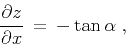 |
(59) |
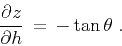 |
(60) |
Equation (A-9) is the basis of the angle-gather construction of
Sava and Fomel (2003).
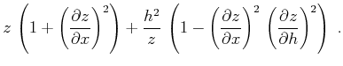
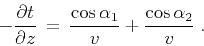
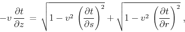
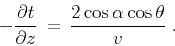
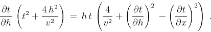
Substituting formulas (A-8) and (A-9) into equation
(A-7) yields yet another form of the double-square-root equation:
![\begin{displaymath}
- {{\partial t} \over {\partial z}} \,=\, {2 \over {v}}\,
\l...
...left({\partial z} \over {\partial h}\right)^2}\right]^{-1}\;,
\end{displaymath}](img146.png) |
(61) |
which is analogous to the dispersion relationship of Stolt prestack
migration (Stolt, 1978).
The law of sines in the triangle formed by the incident and reflected
ray leads to the explicit relationship between the traveltime and the
offset:
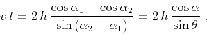 |
(62) |
An algebraic combination of formulas (A-11), (A-5), and
(A-6) forms the basic kinematic equation of the offset
continuation theory (Fomel, 2003a):
 |
(63) |
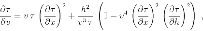
Differentiating (A-11) with respect to the velocity yields
 |
(64) |
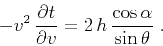
Finally, dividing (A-13) by (A-7) produces
 |
(65) |
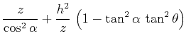
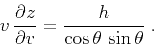
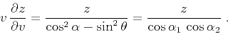
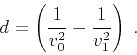
Equation (A-14) can be written in a variety of ways with the help
of an explicit geometric relationship between the half-offset  and
the depth ,
and
the depth ,
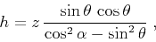 |
(66) |
which follows directly from the trigonometry of the triangle in Figure
A-1 (Fomel, 2003a). For example, equation (A-14) can
be transformed to the form obtained by Liu and Bleistein (1995):
 |
(67) |
In order to separate different factors contributing to the velocity
continuation process, one can transform this equation to the form
Rewritten in terms of the vertical traveltime  , it further
transforms to equation
, it further
transforms to equation
 |
(69) |
equivalent to equation (1) in the main text. Yet
another form of the kinematic velocity continuation equation follows
from eliminating the reflection angle  from equations
(A-14) and (A-15). The resultant expression takes the
following form:
from equations
(A-14) and (A-15). The resultant expression takes the
following form:
 |
(70) |
Appendix
B
Derivation of the residual DMO kinematics
This appendix derives the kinematical laws for the residual NMO+DMO
transformation in the prestack offset continuation process.
The direct solution of equation (31) is
nontrivial. A simpler way to obtain this solution is to decompose
residual NMO+DMO into three steps and to evaluate their contributions
separately. Let the initial data be the zero-offset reflection event
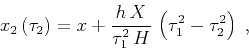
 . The first step of the residual NMO+DMO is the inverse
DMO operator. One can evaluate the effect of this operator by means of
the offset continuation concept (Fomel, 2003a). According to this
concept, each point of the input traveltime curve
travels with the change of the offset from zero to along a special
trajectory, which I call a time ray. Time rays are parabolic
curves of the form
. The first step of the residual NMO+DMO is the inverse
DMO operator. One can evaluate the effect of this operator by means of
the offset continuation concept (Fomel, 2003a). According to this
concept, each point of the input traveltime curve
travels with the change of the offset from zero to along a special
trajectory, which I call a time ray. Time rays are parabolic
curves of the form
 |
(71) |
with the final points constrained by the equation
 |
(72) |
where
 is the derivative of
 .
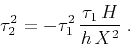
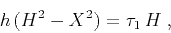
The second step of the cumulative residual NMO+DMO process is the
residual normal moveout. According to equation (23), residual
NMO is a one-trace operation transforming the traveltime
.
The second step of the cumulative residual NMO+DMO process is the
residual normal moveout. According to equation (23), residual
NMO is a one-trace operation transforming the traveltime  to
to
 as follows:
 |
(73) |
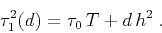
where
 |
(74) |
The third step is dip moveout corresponding to the new velocity
 . DMO is the offset continuation from to zero
offset along the redefined time rays (Fomel, 2003a)
. DMO is the offset continuation from to zero
offset along the redefined time rays (Fomel, 2003a)
 |
(75) |
where
 , and
, and
 .
The end points of the time rays (B-5) are defined by the
equation
.
The end points of the time rays (B-5) are defined by the
equation
 |
(76) |
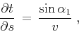
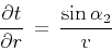
The partial derivatives of the common-offset traveltimes are
constrained by the offset continuation kinematic equation
 |
(77) |
which is equivalent to equation (A-12) in Appendix
A. Additionally, as follows from equations (B-3) and the ray
invariant equations from (Fomel, 2003a),
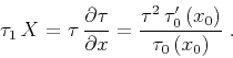 |
(78) |
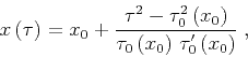
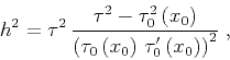
Substituting (B-1-B-4) and
(B-7-B-8) into equations
(B-5) and (B-6) and performing the algebraic
simplifications yields the parametric expressions for velocity
rays of the residual NMO+DMO process:
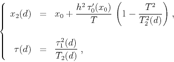 |
(79) |
where the function
 is defined by
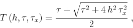 |
(80) |
 |
(81) |
and
 |
(82) |
The last step of the cascade of inverse DMO, residual NMO, and DMO is
illustrated in Figure B-1. The three plots in the figure show
the offset continuation to zero offset of the inverse DMO impulse
response shifted by the residual NMO operator. The middle plot
corresponds to zero NMO shift, for which the DMO step collapses the
wavefront back to a point. Both positive (top plot) and negative
(bottom plot) NMO shifts result in the formation of the specific
triangular impulse response of the residual NMO+DMO operator. As
noticed by Etgen (1990), the size of the triangular
operators dramatically decreases with the time increase. For large
times (pseudo-depths) of the initial impulses, the operator collapses
to a point corresponding to the pure NMO shift.
vlcvoc
Figure B-1. Kinematic residual NMO+DMO
operators constructed by the cascade of inverse DMO, residual NMO,
and DMO. The impulse response of inverse DMO is shifted by the
residual NMO procedure. Offset continuation back to zero offset
forms the impulse response of the residual NMO+DMO operator. Solid
lines denote traveltime curves; dashed lines denote the offset
continuation trajectories (time rays). Top plot:  .
Middle plot: .
Middle plot:  ; the inverse DMO impulse response
collapses back to the initial impulse. Bottom plot: ; the inverse DMO impulse response
collapses back to the initial impulse. Bottom plot:  .
The half-offset in all three plots is 1 km. .
The half-offset in all three plots is 1 km.
|

|
![[sage]](icons/sage.png)
|
|---|
Appendix
C
INTEGRAL VELOCITY CONTINUATION AND KIRCHHOFF MIGRATION
The main goal of this appendix is to prove the equivalence between the
result of zero-offset velocity continuation from zero velocity and
conventional post-stack migration. After solving the velocity
continuation problem in the frequency domain, I transform the solution
back to the time-and-space domain and compare it with the conventional
Kirchhoff migration operator (Schneider, 1978). The frequency-domain
solution has its own value, because it forms the basis for an efficient
spectral algorithm for velocity continuation (Fomel, 2003b).
Zero-offset migration based on velocity continuation is the solution
of the boundary problem for equation (41) with the
boundary condition
 |
(83) |
where  is the zero-offset seismic section, and
 is the continued wavefield. In order to find the solution
of the boundary problem composed of (41) and
(C-1), it is convenient to apply the function
transformation
is the continued wavefield. In order to find the solution
of the boundary problem composed of (41) and
(C-1), it is convenient to apply the function
transformation
 , the time coordinate
transformation
, the time coordinate
transformation
 , and, finally, the double Fourier
transform over the squared time coordinate
, and, finally, the double Fourier
transform over the squared time coordinate  and the spatial
coordinate
and the spatial
coordinate  :
:
 |
(84) |
With the change of domain, equation (41) transforms
to the ordinary differential equation
 |
(85) |
and the boundary condition (C-1) transforms to the initial
value condition
 |
(86) |
where
 |
(87) |
and
 . The unique solution of the initial value
(Cauchy) problem (C-3) - (C-4) is easily found to be
. The unique solution of the initial value
(Cauchy) problem (C-3) - (C-4) is easily found to be
 |
(88) |
In the transformed domain, velocity continuation appears to be a unitary
phase-shift operator. An immediate consequence of this remarkable fact is the
cascaded migration decomposition of post-stack migration
(Larner and Beasley, 1987):
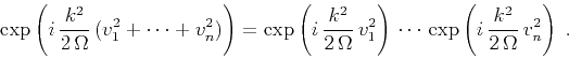 |
(89) |
Analogously, three-dimensional post-stack migration is decomposed
into the two-pass procedure (Jakubowicz and Levin, 1983):
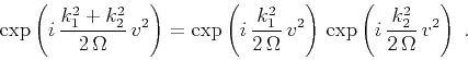 |
(90) |
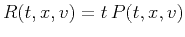
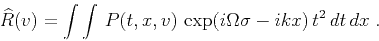
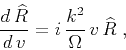
The inverse double Fourier transform of both sides of equality
(C-6) yields the integral (convolution) operator
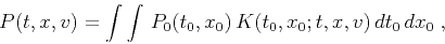 |
(91) |
with the kernel  defined by
 |
(92) |
where  is the number of dimensions in and
  ( equals
  or
or  ). The inner integral on the wavenumber axis in formula
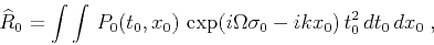
(C-10) is a known table integral (Gradshtein and Ryzhik, 1994). Evaluating this
integral simplifies equation (C-10) to the form
). The inner integral on the wavenumber axis in formula
(C-10) is a known table integral (Gradshtein and Ryzhik, 1994). Evaluating this
integral simplifies equation (C-10) to the form
![\begin{displaymath}
K = {{t_0^2/t} \over {(2\,\pi)^{m/2+1}\,v^m}}\,
\int\,(i\Ome...
...2 - t^2 - {{(x - x_0)^2} \over v^2}\right)\right]\,
d\Omega\;.
\end{displaymath}](img197.png) |
(93) |
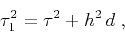
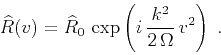
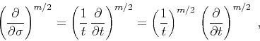
The term
 is the spectrum of the anti-causal
derivative operator
is the spectrum of the anti-causal
derivative operator
 of the order
  . Noting
the equivalence
. Noting
the equivalence
 |
(94) |
which is exact in the 3-D case ( ) and asymptotically correct in
the 2-D case (
) and asymptotically correct in
the 2-D case ( ), and applying the convolution theorem
transforms operator (C-9) to the form
), and applying the convolution theorem
transforms operator (C-9) to the form
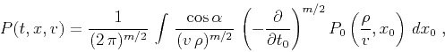 |
(95) |
where
 , and
, and
 . Operator (C-13) coincides with the Kirchhoff operator
of conventional post-stack time migration (Schneider, 1978).
. Operator (C-13) coincides with the Kirchhoff operator
of conventional post-stack time migration (Schneider, 1978).
|
|
|
|
| Velocity continuation and the anatomy of
residual prestack time migration | |
|
Next: About this document ...
Up: Fomel: Velocity continuation
Previous: Acknowledgments
2014-04-01