|
|
|
|
Time migration velocity analysis by velocity continuation |
After the velocity continuation process has created a time-midpoint-velocity cube, one can pick the best focusing velocity from that cube and create an optimally focused image by slicing through the cube. This step is common in other methods that involve velocity slicing (Fowler, 1984; Mikulich and Hale, 1992; Shurtleff, 1984). The algorithm described below has been also adopted by Sava (2000) for velocity analysis in wave-equation migration.
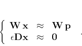
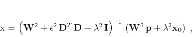
A simple automatic velocity picking algorithm follows from solving the
following regularized least-squares system:
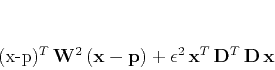
In the case of picking a one-dimensional velocity function from a single
semblance panel, one can simplify the algorithm by choosing ![]() to be a
convolution with the derivative filter
to be a
convolution with the derivative filter ![]() . It is easy to see that in
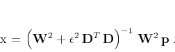
this case the inverted matrix in formula (17) has a tridiagonal
structure and therefore can be easily inverted with a linear-time algorithm.
The regularization parameter
. It is easy to see that in
this case the inverted matrix in formula (17) has a tridiagonal
structure and therefore can be easily inverted with a linear-time algorithm.
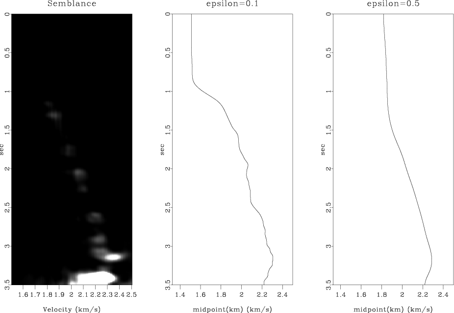
The regularization parameter ![]() controls the amount of smoothing of
the estimated velocity function. Figure 10 shows an example
velocity spectrum and two automatic picks for different values of
controls the amount of smoothing of
the estimated velocity function. Figure 10 shows an example
velocity spectrum and two automatic picks for different values of ![]() .
.
|
|---|
|
velpick
Figure 10. Semblance panel (left) and automatic velocity picks for different values of the regularization parameter. Higher values of |
|
|
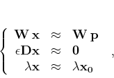
In the case of picking two- or three-dimensional velocity functions,
one could generalize problem (15) by defining ![]() as a 2-D or 3-D roughening operator. I chose to use a more simplistic
approach, which retains the one-dimensional structure of the algorithm.
I transform system (15) to the form
as a 2-D or 3-D roughening operator. I chose to use a more simplistic
approach, which retains the one-dimensional structure of the algorithm.
I transform system (15) to the form
After the velocity has been picked, an optimally focused image is constructed by slicing in the time-midpoint-velocity cube. I used simple linear interpolation for slicing between the velocity grid values. A more accurate interpolation technique can be easily adopted.
|
|
|
|
Time migration velocity analysis by velocity continuation |