|
|
|
|
Automatic traveltime picking using the instantaneous traveltime |


|
|---|
|
syn,ltf0,tt0
Figure 2. (a) Synthetic signal. (b) Local The dashed lines in (b) and (c) indicate the effective bandwidth (estimated using equation 11). |
|
|
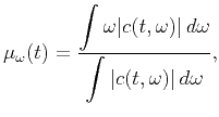
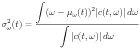
For most data, the bandwidth of signals is varying with time. It therefore makes sense to estimate the effective bandwidth as a function of time. In order to choose the frequency band automatically, we suggest any data-driven criterion, such as an estimate of the instantaneous frequency or some weighted mean of the frequency. An obvious choice is
The result of the averaging operation is shown in Figure 3(b), in which
![]() is averaged over the frequencies in its effective bandwidth. (Figure 3(a) is the same as Figure 2(a) and shown here just to illustrate the agreement between the actual arrivals and the picked arrivals.) Parameter
is averaged over the frequencies in its effective bandwidth. (Figure 3(a) is the same as Figure 2(a) and shown here just to illustrate the agreement between the actual arrivals and the picked arrivals.) Parameter ![]() equals the recording
equals the recording ![]() (dashed line) at the times of arrival of the spikes, namely at
(dashed line) at the times of arrival of the spikes, namely at
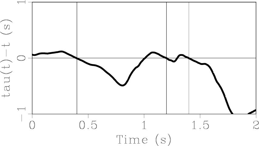
![]() , 1.1991 and 1.3978 s. It should be noted that although there are actually no arrivals between two consecutive arrivals,
, 1.1991 and 1.3978 s. It should be noted that although there are actually no arrivals between two consecutive arrivals, ![]() is not zero in that interval. This is due to the smooth division we employed, when dividing
is not zero in that interval. This is due to the smooth division we employed, when dividing
![]() over
over ![]() . Smooth division does not allow the result to vary erratically from sample to sample.
Figure 3(c) shows the difference
. Smooth division does not allow the result to vary erratically from sample to sample.
Figure 3(c) shows the difference ![]() . This difference equals 0 at the times of arrival of the two spikes.
However not all zeros of
. This difference equals 0 at the times of arrival of the two spikes.
However not all zeros of ![]() are of interest; rather, only the zero crossings from positive to negative values yield valid traveltimes. Positive maxima of
are of interest; rather, only the zero crossings from positive to negative values yield valid traveltimes. Positive maxima of ![]() (as in
(as in
![]() ) denote an imminent arrival of a signal. Let's assume a strong (compared to neighboring events) event at some time
) denote an imminent arrival of a signal. Let's assume a strong (compared to neighboring events) event at some time ![]() . According to equation 3,
. According to equation 3, ![]() is a weighted some of the times of arrivals around
is a weighted some of the times of arrivals around ![]() . The closer
. The closer ![]() is to the imminent arrival at
is to the imminent arrival at ![]() , the more the value of
, the more the value of ![]() will be biased towards the value
will be biased towards the value ![]() . Therefore
. Therefore ![]() will be greater than
will be greater than ![]() , i.e.,
, i.e.,
![]() . For
. For ![]() , the value of
, the value of ![]() will still be biased towards
will still be biased towards ![]() , therefore
, therefore
![]() . In fact, the higher the energy of the arriving signal at some time
. In fact, the higher the energy of the arriving signal at some time ![]() compared with that of neighboring events, the closer the value of
compared with that of neighboring events, the closer the value of ![]() to
to ![]() will be.
Accordingly, an event is identified by the non-zero values of the function
will be.
Accordingly, an event is identified by the non-zero values of the function

|
|---|
|
syn0,taut0,tau-t0
Figure 3. (a) Synthetic signal (sampling period is 4 ms). Arrivals are at 0.4, 1.2 and 1.4 s. (b) |
|
|
|
|
|
|
Automatic traveltime picking using the instantaneous traveltime |