Acoustic wavefield evolution as function of source location perturbation

The Green's function

The Green's function represents the response and behavior of the wavefield if the source was a point impulse given theoretically by the Dirac delta function. The function allows us to solve the wave equation using an integral formulation as we convolve the Green's function with a source function. The most complicated part of this type of solution of the wave equation is the construction of the Green's function. Kirchhoff modeling and migration is a special case of this type of integral solution and provides incredible speed upgrades over finite difference implementations with some loss in quality, because of the limitations in the calculation of the phase and amplitude components of the Green's function.

Since Green's function for the wave equation satisfies the following formula:

$$\frac{\partial^2 G}{\partial x^2}+ \frac{\partial^2 G}{\partial y... ...x,y,z) \frac{\partial^2 G}{\partial t^2} + \delta({\bf {x-x_0}}) \delta(t-t_0),$$ (9)

where $\delta$ is the Dirac delta function, with $\bf {x_0}$ ($x_0$, $y_0$, $z_0$), and $t_0$ is the possible location and time of the source pulse, respectively. The solution of equation (1) with a source function $f({\bf {x_0}},t_0)$ is given by

$$u(x,y,z,t) = \int \int G({\bf {x,x_0}},t,t_0) f({\bf {x_0}},t_0) d{\bf {x_0}} dt_0.$$ (10)

In typical imaging applications, the Green's function is evaluated upfront and stored in tables for use in prestack modeling and migration. For source perturbations, these stored Green's functions can be used to approximate the wavefield for a shift in the source location by using a source function that is based on Taylor's series expansion, without the need to modify the Green's function. Specifically, considering that in the first-order perturbation equation (4):

$$f_l(x,y,z,t)= - \frac{\partial w}{\partial x} \frac{\partial^2 u}{\partial t^2},$$ (11)

then since equation (4) has the same form as the wave equation with the same velocity function,

$$D_x(x,y,z,t) = \int \int G({\bf {x,x_0}},t,t_0) f_l({\bf {x_0}},t_0) d{\bf {x_0}} dt_0.$$ (12)

The same argument holds for the second-order perturbation equation (7) with a slightly more complicated source function given by

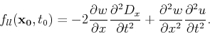$$f_{ll}({\bf {x_0}},t_0) = - 2 \frac{\partial w}{\partial x} ... ...\partial^2 w}{\partial x^2} \frac{\partial^2 u}{\partial t^2}.$$ (13)

Thus, the wavefield form can be approximated for a source perturbed a distance $l$ using

$$u(x,y,z,l,t) \approx \int \int G({\bf {x,x_0}},t,t_0) \left(f({\b... ..._0}},t_0) l + \frac{1}{2} f_{ll}({\bf {x_0}},t_0) l^2\right) d{\bf {x_0}} dt_0.$$ (14)

Thus, the wavefield corresponding to a certain source location can be directly evaluated using the background Green's function with a modified source function, and these modifications, unlike the conventional ones, are dependent on lateral velocity variations.

Acoustic wavefield evolution as function of source location perturbation