Structure-constrained relative acoustic impedance using stratigraphic coordinates

example

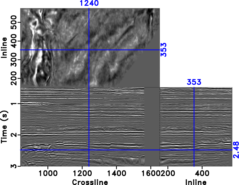
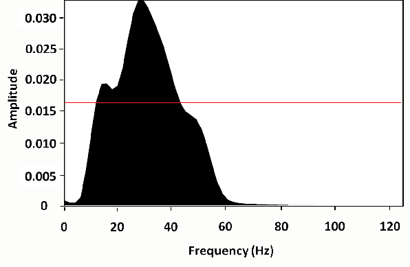
I use a 3D field data volume from Heidrun Field in the Halten Terrace area, offshore Mid-Norway (Moscardelli et al., 2013) to test the proposed approach (Figure 1a). I begin by estimating local slopes of seismic events through the data volume using plane-wave destruction. After that, I apply the predictive painting algorithm to obtain the first axis of the stratigraphic coordinates. The two other axes are found by solving gradient equations 6 and 7. Figure 1b shows the image in the Cartesian coordinate system, overlain by its stratigraphic coordinates grid. Figure 1c shows the image in the stratigraphic coordinate system, where major reflectors appear nearly flat, and Figure 1d displays the image reconstruction by returning from stratigraphic coordinates to Cartesian coordinates. I use model-based inversion (Russell and Hampson, 1991; Cooke and Schneider, 1983) to extract acoustic impedance information from the seismic image. Because of the band-limited nature of seismic data, low-frequency variations are extracted from the well data, and then added back to the seismic data in order to obtain a proper broad-band result. Model-based inversion starts with a low-frequency model of P-impedance and perturbs this model until the derived synthetic section from the application of equations 1 and 2 best fits the actual seismic data. In the model-based inversion, extraction of the seismic wavelet is necessary. Figure 2 shows the extracted wavelet from the seismic image in the Cartesian coordinates, Figure 2a is the time response, and Figure 2b is the frequency response of the seismic wavelet. Figure 3 shows the extracted wavelet from the seismic image in the stratigraphic coordinate system.

Figure 4a is a zoomed-in part of the image, and Figure 4b is the impedance results obtained from inversion in the Cartesian coordinates. Figure 4c shows the impedance inversion result acquired in the stratigraphic coordinate system and transferred back to Cartesian coordinate system to provide a better comparison. Comparing the impedance acquired from inversion in the conventional Cartesian coordinates (Figures 4b) with the result obtained from inversion in the stratigraphic coordinates (Figures 4c) shows that result from inversion in stratigraphic coordinates (Figures 4c) appears to be more consistent with the geological structure and also more detailed. Interfaces are noticeably better defined and laterally more continuous. This improved accuracy result because, in the stratigraphic coordinates, layers get flattened and the vertical direction corresponds to the normal direction to reflectors, and therefore allows for a more accurate analysis of the earth's normal incidence reflectivity and its impedance.

stack,coord,hcubee,hcubeee
Figure 1. (a) 3D field data from Heidrun. (b) Three axes of stratigraphic coordinates of Figure 1a plotted as grid in their Cartesian coordinates. (c) Heidrun image after flattening by transferring the image to stratigraphic coordinates. (d) Heidrun image reconstruction by returning from stratigraphic coordinates to Cartesian coordinates.

t-car-full,f-car-full
Figure 2. Extracted wavelet from the seismic data in Figure 1a in the Cartesian coordinates, (a) is the time response and (b) is the frequency response.

t-st-full,f-st-full
Figure 3. Extracted wavelet from the seismic data in Figure 1c in the stratigraphic coordinates, (a) is the time response and (b) is the frequency response.

inline-331-sei-mod-1,inline-331-car-mod-1,inline-331-st-mod-1
Figure 4. (a) A zoomed-in part of the Figure 1a and the impedance result obtained from inversion in the Cartesian coordinates (b), and in the stratigraphic coordinates (the result is transferred back to Cartesian coordinates to provide a better comparison) (c).

Structure-constrained relative acoustic impedance using stratigraphic coordinates