 |
 |
 |
 | Seismic data interpolation beyond aliasing using regularized nonstationary autoregression |  |
![[pdf]](icons/pdf.png) |
Next: Missing data interpolation
Up: Step 1: Adaptive PEF
Previous: Step 1: Adaptive PEF
An important property of PEFs is scale invariance, which allows
estimation of PEF coefficients  (including the leading ``
 ''
and prediction coefficients
''
and prediction coefficients  ) for incomplete aliased data
 that include known traces
 and unknown or zero traces
 . For trace decimation, zero
traces interlace known traces. To avoid zeroes that influence filter
estimation, we interlace the filter coefficients with zeroes. For
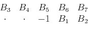
example, consider a 2-D PEF with seven prediction coefficients:
. For trace decimation, zero
traces interlace known traces. To avoid zeroes that influence filter
estimation, we interlace the filter coefficients with zeroes. For
example, consider a 2-D PEF with seven prediction coefficients:
 |
(1) |
Here, the horizontal axis is time, the vertical axis is space, and
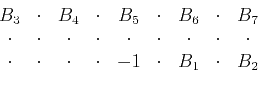
`` '' denotes zero. Rescaling both time and spatial axes assumes
that the dips represented by the original filter in
equation 1 are the same as those represented by the
scaled filter
(Claerbout, 1992):
'' denotes zero. Rescaling both time and spatial axes assumes
that the dips represented by the original filter in
equation 1 are the same as those represented by the
scaled filter
(Claerbout, 1992):
 |
(2) |
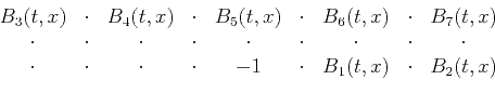
For nonstationary situations, we can also assume locally stationary
spectra of the data because trace decimation makes the space between
known traces small enough, thus making adaptive PEFs locally
scale-invariant. For estimating adaptive PEF coefficients,
nonstationary autoregression allows coefficients
to change with
both  and
and  . The new adaptive filter can look something like
 |
(3) |
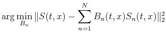
In other words, prediction coefficients  are
obtained by solving the least-squares problem,
are
obtained by solving the least-squares problem,
where  =
=
 , which
represents the causal translation of
, with time-shift index
, which
represents the causal translation of
, with time-shift index
 and spatial-shift index
  scaled by decimation interval
 . Note that predefined constant
uses the interlacing value as
an interval; i.e., the shift interval equals 2 in
equation 3. Subscript
. Note that predefined constant
uses the interlacing value as
an interval; i.e., the shift interval equals 2 in
equation 3. Subscript  is the general shift index
for both time and space, and the total number of
and
is
is the general shift index
for both time and space, and the total number of
and
is
 .
.
 is the regularization operator, and
  is a
scalar regularization parameter. All coefficients
are
estimated simultaneously in a time/space variant manner. This approach
was described by Fomel (2009) as regularized nonstationary
autoregression (RNA). If
is a linear operator,
least-squares estimation reduces to linear inversion
is a
scalar regularization parameter. All coefficients
are
estimated simultaneously in a time/space variant manner. This approach
was described by Fomel (2009) as regularized nonstationary
autoregression (RNA). If
is a linear operator,
least-squares estimation reduces to linear inversion
 |
(5) |
where
![$\displaystyle \mathbf{b} = \left[\begin{array}{cccc}B_1(t,x) & B_2(t,x) & \cdots & B_N(t,x)\end{array}\right]^T\;,$](img36.png) |
(6) |
![$\displaystyle \mathbf{d} = \left[\begin{array}{cccc}S_1(t,x)\,S(t,x) & S_2(t,x)\,S(t,x) & \cdots & S_N(t,x)\,S(t,x)\end{array}\right]^T\;,$](img37.png) |
(7) |
and the elements of matrix
 are
are
 |
(8) |
Shaping regularization (Fomel, 2007) incorporates a shaping
(smoothing) operator
 instead of
and
provides better numerical properties than Tikhonov's
regularization (Tikhonov, 1963) in
equation 4 (Fomel, 2009).
Inversion using shaping regularization takes the form
instead of
and
provides better numerical properties than Tikhonov's
regularization (Tikhonov, 1963) in
equation 4 (Fomel, 2009).
Inversion using shaping regularization takes the form
 |
(9) |
where
![$\displaystyle \widehat{\mathbf{d}} = \left[\begin{array}{cccc}\mathbf{G}\left[S...
...ight] & \cdots & \mathbf{G}\left[S_N(t,x)\,S(t,x)\right]\end{array}\right]^T\;,$](img42.png) |
(10) |
the elements of matrix
 are
are
and  is a scaling coefficient. One advantage of the shaping
approach is the relative ease of controlling the selection of
and
in comparison with
and
. We define
as Gaussian smoothing with an
adjustable radius, which is designed by repeated application of
triangle smoothing (Fomel, 2007), and choose
to be the
mean value of
.
is a scaling coefficient. One advantage of the shaping
approach is the relative ease of controlling the selection of
and
in comparison with
and
. We define
as Gaussian smoothing with an
adjustable radius, which is designed by repeated application of
triangle smoothing (Fomel, 2007), and choose
to be the
mean value of
.
Coefficients
 at zero traces
get constrained
(effectively smoothly interpolated) by regularization. The required
parameters are the size and shape of the filter
and the
smoothing radius in
.
at zero traces
get constrained
(effectively smoothly interpolated) by regularization. The required
parameters are the size and shape of the filter
and the
smoothing radius in
.
|
|
|
|
| Seismic data interpolation beyond aliasing using regularized nonstationary autoregression | |
|
Next: Missing data interpolation
Up: Step 1: Adaptive PEF
Previous: Step 1: Adaptive PEF
2013-07-26
![$\displaystyle + \epsilon^2\, \sum_{n=1}^{N} \Vert\mathbf{D}[B_n(t,x)]\Vert _2^2\;,$](img25.png)