|
|
|
|
Application of spectral decomposition using regularized non-stationary autoregression to random noise attenuation |
Next: Discussions Up: Yang et al.: Denoising Previous: Algorithm steps
|
|
|
|
Application of spectral decomposition using regularized non-stationary autoregression to random noise attenuation |

|
|---|
|
trace-disp
Figure 3. Denoising demonstration using the proposed approach for single-trace synthetic data. (a) Noisy data. (b) First spectral component. (c) Second spectral component. (d) Third spectral component. (e) Fourth spectral component. (f) The residual after SDRNAR. (g) Denoised data. The SNR has increased from -10.17 to 0.9729. |
|
|
The first example is a noisy single trace, shown in Figure 3a. The clean synthetic trace is generated by convolving Ricker wavelet with four different central frequency (40 Hz, 30 Hz, 20 Hz, and 10Hz, respectively) with the same reflectivity coefficients located at different temporal positions. After adding Gaussian white noise, the wavelet has been smeared in the noise. After spectral decomposition using SDRNAR, the decomposed signals are shown in Figures 3b-3e. The residual or the random noise is shown in Figure 3f. The denoised data, summation of 3b-3e, is shown in Figure 3g. A huge level of noise has been removed during the denoising process. In order to numerically compare the performances using the proposed approach, we use the signal-to-noise ratio (SNR) defined as:
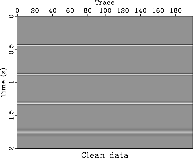
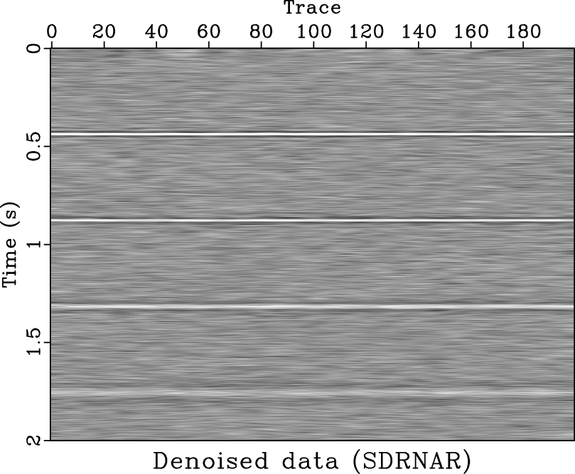
The second example is a synthetic seismic profile with four horizontal events (Figures 4). Figures 4a and 4b show the clean and noisy synthetic data, respectively. The central frequency of the Ricker wavelet used to synthesize the profile is decreasing as we can see from the original profile. Their corresponding central frequency are 40Hz, 30Hz, 20 Hz, and 10 Hz, from up to down, respectively. The denoised section and removed noise section are shown in Figures 5a and 5b, respectively. As a reference, Figures 5c and 5d show the denoised profile and removed noise section for ![]() -
-![]() deconvolution. Because of the application of spatial prediction filter in
deconvolution. Because of the application of spatial prediction filter in ![]() -
-![]() domain, there exist some boundary effects in the denoised section, as shown in Figure 5c. The clean denoised section and coherency-free noise sections using the proposed approach show an excellent denoising performance.
domain, there exist some boundary effects in the denoised section, as shown in Figure 5c. The clean denoised section and coherency-free noise sections using the proposed approach show an excellent denoising performance.
The original SNR of the noisy data (Figure 4b) is ![]() . After using
. After using ![]() -
-![]() deconvolution (5c), the SNR increases to
deconvolution (5c), the SNR increases to ![]() . After using the proposed approach (5a), the SNR increases to
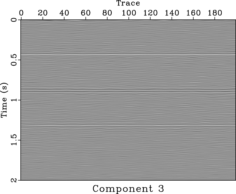
. After using the proposed approach (5a), the SNR increases to ![]() . In this example, we decompose the signal into four components. Figure 6 shows the decomposed four components using SDRNAR. For comparison with EMD, we also demonstrate the four decomposed components using EMD in Figure 7. As can be seen in Figure 6, the decomposed components are clean, exhibiting smoothly-variable frequency. However, the EMD decomposed components have serious mode-mixing issues, as mentioned in (Kopecky, 2010; Chen and Ma, 2014), which made the removal of random noise by removing one mode difficult. The amplitude maps of instantaneous frequency are shown in Figure 8. Figure 8 also confirms the observation from Figure 6 that the decomposed components contain smoothly-variable frequency.
. In this example, we decompose the signal into four components. Figure 6 shows the decomposed four components using SDRNAR. For comparison with EMD, we also demonstrate the four decomposed components using EMD in Figure 7. As can be seen in Figure 6, the decomposed components are clean, exhibiting smoothly-variable frequency. However, the EMD decomposed components have serious mode-mixing issues, as mentioned in (Kopecky, 2010; Chen and Ma, 2014), which made the removal of random noise by removing one mode difficult. The amplitude maps of instantaneous frequency are shown in Figure 8. Figure 8 also confirms the observation from Figure 6 that the decomposed components contain smoothly-variable frequency.
The third example is a relatively more complex data, with dipping and conflicting events (Figure 9). This example demonstrates the limitation of the proposed approach in dealing with complex seismic profiles. As we can see from the both denoised section and removed noise section as shown in Figures 9b and 9c, respectively, there is some damages to dipping energy. As the slope becomes larger, there are more damages to the useful energy. The horizontal events, however, are well preserved and denoised. The reason causing the limitation of the proposed approach comes from the fact that the SDRNAR method is applied trace by trace. The parameters selected for the decomposition should be relatively the same in order to be efficient, otherwise, we need to specify the parameters trace by trace, which make the SDRNAR method can not adapt to highly spatially variable components, e.g., steeply dipping event. We also show the performance of the same example using the mean filter. Figure 9d is the denoised result using mean filter and Figure 9e is the corresponding noise section. As we can see from Figures 9d and 9e, the mean filter nearly remove all the dipping energy.
The fourth example is a post-stack field data. It comes from part of the 2-D field land data from the open-source website Freeusp
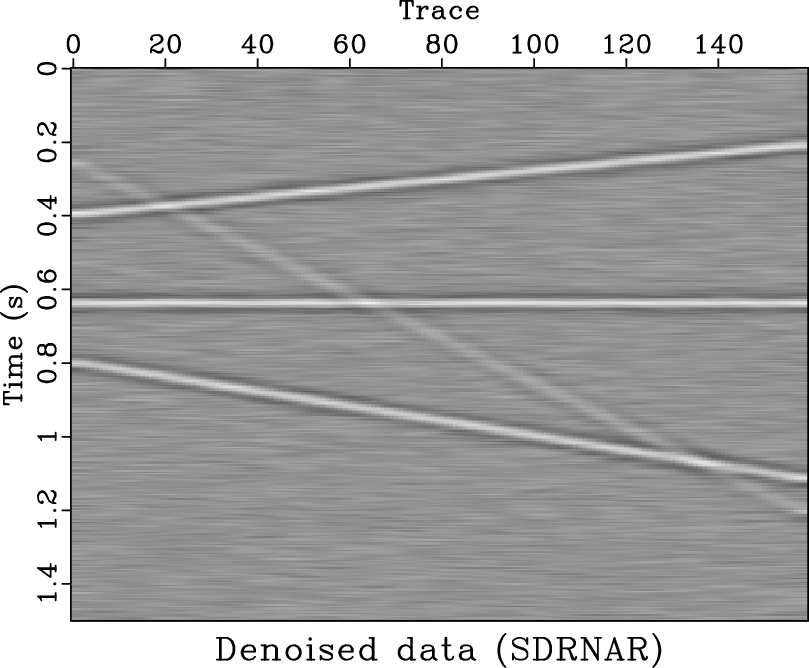
(http://www.freeusp.org/). The stacked data is shown in Figure 10. After random noise attenuation using the proposed approach, the denoised data is shown in Figure 11a. Figure 11b shows the difference between the denoised section and original noise section. From the denoising performance, we conclude the proposed approach does an excellent job. We also apply ![]() -
-![]() deconvolution and mean filter to the field dataset. The denoised section and removed noise section using
deconvolution and mean filter to the field dataset. The denoised section and removed noise section using ![]() deconvolution are shown in Figure 11c and 11d, respectively. The denoised section and removed noise section using mean filter are shown in Figure 11e and 11f, respectively. Even though the denoised section using
deconvolution are shown in Figure 11c and 11d, respectively. The denoised section and removed noise section using mean filter are shown in Figure 11e and 11f, respectively. Even though the denoised section using ![]() -
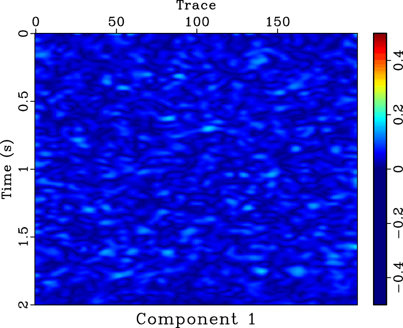
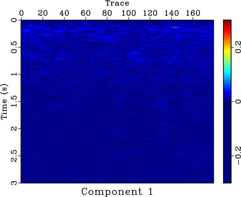
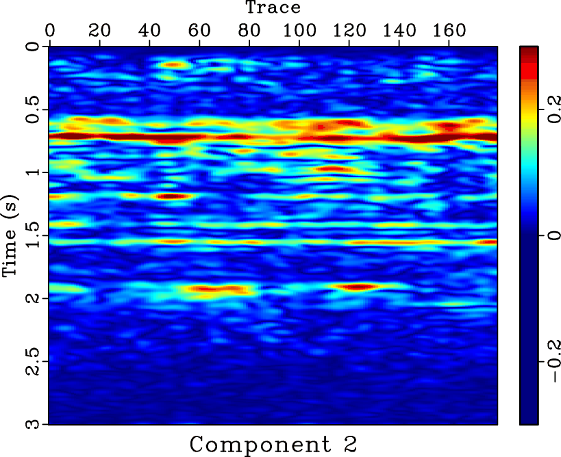
-![]() deconvolution and mean filter seem clean, there exist some coherent horizontal events in the noise section (Figures 11d and 11f). Because in this example we do not know the true answer, we can not numerically compare the SNRs of two approaches, however, from the visual comparisons, it is enough to draw a conclusion that the proposed approach does a better job. In this example, the denoised section using mean filter is over smoothed. The two areas pointed out by the labels A and B show the over-smoothed places. The spatial discontinuities will cause a failure using mean filter because mean filter is based on the spatial coherency assumption. The lost information due to over smoothing can be found in the noise section, as pointed out by the label C. Thus, we conclude that the proposed approach can outperform the mean filter in preserving spatial discontinuities. Figure 12 shows the four decomposed components using SDRNAR, from which we can see the smoothly-variable-frequency behavior for each component. For a referential comparison, the separated results using EMD are shown in Figure 13. It is obvious that the separated components do not have constant or smoothly-variable frequency. Additionally, we obtain the spectral information shown in Figure 14. From Figure 14d, it seems that there is a low-frequency anomaly around 0.75 s, which may indicate a trap of oil & gas.
deconvolution and mean filter seem clean, there exist some coherent horizontal events in the noise section (Figures 11d and 11f). Because in this example we do not know the true answer, we can not numerically compare the SNRs of two approaches, however, from the visual comparisons, it is enough to draw a conclusion that the proposed approach does a better job. In this example, the denoised section using mean filter is over smoothed. The two areas pointed out by the labels A and B show the over-smoothed places. The spatial discontinuities will cause a failure using mean filter because mean filter is based on the spatial coherency assumption. The lost information due to over smoothing can be found in the noise section, as pointed out by the label C. Thus, we conclude that the proposed approach can outperform the mean filter in preserving spatial discontinuities. Figure 12 shows the four decomposed components using SDRNAR, from which we can see the smoothly-variable-frequency behavior for each component. For a referential comparison, the separated results using EMD are shown in Figure 13. It is obvious that the separated components do not have constant or smoothly-variable frequency. Additionally, we obtain the spectral information shown in Figure 14. From Figure 14d, it seems that there is a low-frequency anomaly around 0.75 s, which may indicate a trap of oil & gas.

|
|---|
|
synth0,synth
Figure 4. (a) Clean synthetic data. (b) Noisy synthetic data. |
|
|


|
|---|
|
synth-cfit,synth-cdif,synth-fx,synth-fx-dif
Figure 5. Amplitudes of different frequency components. |
|
|


|
|---|
|
synth-sign0,synth-sign1,synth-sign2,synth-sign3
Figure 6. Amplitudes of different frequency components. |
|
|


|
|---|
|
simf1,simf2,simf3,simf4
Figure 7. Different separated components for synthetic data using EMD. (a) First separated component. (b) Second separated component. (c) Third separated component. (d) Fourth separated component. |
|
|


|
|---|
|
synth-cwht0,synth-cwht1,synth-cwht2,synth-cwht3
Figure 8. Amplitudes of different frequency components. |
|
|


|
|---|
|
complex,complex-cfit,complex-cdif,complex-mf,complex-mf-dif
Figure 9. (a) Noisy synthetic example with dipping events. (b) Denoised result using the proposed approach. (c) Removed noise section using the proposed approach. Note that the damage to dipping events suggest a denoising failure. (d) Denoised result using mean filter. (e) Removed noise section using mean filter. |
|
|

|
|---|
|
data-f
Figure 10. Input noisy field data from Freeusp. |
|
|


|
|---|
|
cfit-f,cdif-f,data-fx,data-fx-dif,data-mf,data-mf-dif
Figure 11. Different separated components for field data using SDRNAR. (a) First separated component. (b) Second separated component. (c) Third separated component. (d) Fourth separated component. |
|
|


|
|---|
|
sign0,sign1,sign2,sign3
Figure 12. Different separated components for field data using SDRNAR. (a) First separated component. (b) Second separated component. (c) Third separated component. (d) Fourth separated component. |
|
|


|
|---|
|
imf1,imf2,imf3,imf4
Figure 13. Different separated components for field data using EMD. (a) First separated component. (b) Second separated component. (c) Third separated component. (d) Fourth separated component. |
|
|


|
|---|
|
cwht0,cwht1,cwht2,cwht3
Figure 14. Amplitudes of different frequency components. |
|
|
|
|
|
|
Application of spectral decomposition using regularized non-stationary autoregression to random noise attenuation |