A fast butterfly algorithm for generalized Radon transforms

Computing the adjoint operator

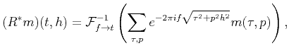
The last example is concerned with the computation of the adjoint of the hyperbolic Radon transform. Assuming $m(\tau,p)$ and $d(t,h)$ are two arbitrary functions (in the discrete sense) in the model domain and data domain, if we require

$$\langle m(\tau,p),(Rd)(\tau,p)\rangle =\langle(R^*m)(t,h),d(t,h)\rangle,$$ (29)

where $(Rd)(\tau,p)$ is given by equation 3, the inner product $\langle\cdot,\cdot\rangle$ is defined as

$$\langle g_1(x,y),g_2(x,y)\rangle\,=\sum_{x,y} g_1(x,y)\,\overline{g_2 (x,y)}, \quad \forall g_1(x,y), \ g_2(x,y);$$ (30)

then it is easy to verify that the adjoint operator $R^*$ is given by

$$(R^*m)(t,h)=\mathcal{F}_{f\rightarrow t}^{-1}\left(\sum_{\tau,p}e^{-2\pi i f \sqrt{\tau^2+p^2h^2}}m(\tau,p)\right),$$ (31)

where $\mathcal{F}^{-1}_{f\rightarrow t}$ is the inverse Fourier transform from variable $f$ to $t$ . The summation in equation 31 again resembles an oscillatory integral operator, therefore the fast algorithm for computing $R$ applies with minor modifications. The computational cost remains the same.

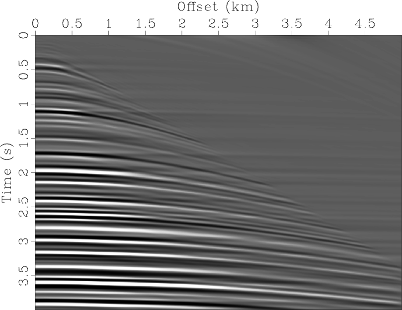
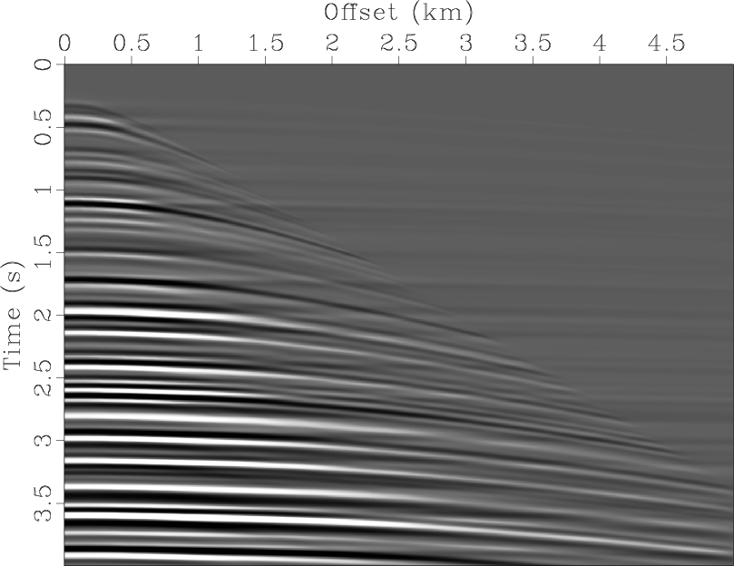
We consider still the first example and apply the (discrete) adjoint operators of the fast butterfly algorithm and the velocity scan respectively to the data in Figures 5 and 6. The two methods produce similar results (see Figures 19, 20). It is also clear that the adjoint is far from the inverse, at least for this geometry, hence some kind of least-squares implementation is needed for inversion process.

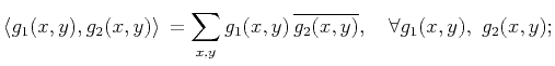
To further verify that the numerically computed $R^*$ is the adjoint operator of $R$ , one can compare the values of $\langle Rd,Rd\rangle$ and $\langle R^*Rd,d\rangle$ for arbitrary $d$ . Indeed, the proposed algorithm passed this dot-product test with a relative error of $O(10^{-7})$ in single precision.

fdat
Figure 19. Output of the adjoint fast butterfly algorithm applied to the data in Figure 5. $N=32$ , $q_{k_1}=q_{k_2}=q_{x_1}=q_{x_2}=9$ .

didat
Figure 20. Output of the adjoint velocity scan applied to the data in Figure 6.

A fast butterfly algorithm for generalized Radon transforms