|
 |
 |
 | Non-hyperbolic common reflection surface |  |
![[pdf]](icons/pdf.png) |
Next: 3-D extension
Up: Fomel & Kazinnik: Nonhyperbolic
Previous: Introduction
If  represents the prestack seismic data as a function of
time
represents the prestack seismic data as a function of
time  , midpoint
  and half-offset
  , then conventional stacking
can be described as
, then conventional stacking
can be described as
 |
(1) |
where  is the stack section, and
 is the
moveout approximation, which may take a form of a hyperbola
is the
moveout approximation, which may take a form of a hyperbola
 |
(2) |
with  as an effective velocity parameter or, alternatively, a more
complicated non-hyperbolic functional form, which involves other
parameters (Fomel and Stovas, 2010).
as an effective velocity parameter or, alternatively, a more
complicated non-hyperbolic functional form, which involves other
parameters (Fomel and Stovas, 2010).
The MF or CRS stacking takes a different form,
 |
(3) |
where the integral over midpoint
is typically carried out only over a limited
neighborhood of  . The multifocusing approximation of
Gelchinsky et al. (1999a) takes the form
. The multifocusing approximation of
Gelchinsky et al. (1999a) takes the form
 |
(4) |
where, in the notation of Tygel et al. (1999),
 |
(5) |
 |
(6) |
and
 |
(7) |
The four parameters
 have clear physical
interpretations in terms of the wavefront and ray geometries
(Gelchinsky et al., 1999a).
have clear physical
interpretations in terms of the wavefront and ray geometries
(Gelchinsky et al., 1999a).  represents the velocity at the surface and is typically
assumed known and constant around the central ray. One important property of the MF
approximation is that, in a constant velocity medium with velocity
, it can
accurately describe both reflections from a plane dipping interfaces and diffractions from point diffractors.
represents the velocity at the surface and is typically
assumed known and constant around the central ray. One important property of the MF
approximation is that, in a constant velocity medium with velocity
, it can
accurately describe both reflections from a plane dipping interfaces and diffractions from point diffractors.
The CRS approximation (Jäger et al., 2001) is
 |
(8) |
where
 , and the three parameters
 are related to the multifocusing parameters as
follows:
are related to the multifocusing parameters as
follows:
Equation (8) is equivalent to a truncated Taylor expansion
of the squared traveltime in equation (4) around  and
and
 . In comparison with MF, CRS possesses a fundamental
simplicity, which makes it easy to extend the method to 3-D. However,
it looses the property of accurately describing diffractions in a
constant-velocity medium.
. In comparison with MF, CRS possesses a fundamental
simplicity, which makes it easy to extend the method to 3-D. However,
it looses the property of accurately describing diffractions in a
constant-velocity medium.
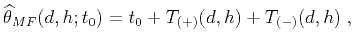
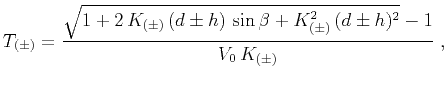
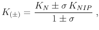
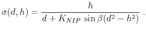
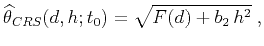
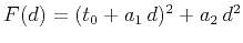
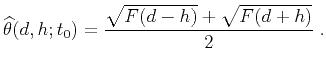
We propose the following modification of approximation (8):
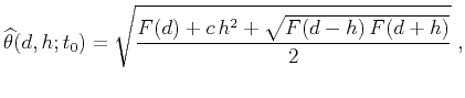 |
(12) |
where
 . Equation (12), which we call
non-hyperbolic common reflection surface, is derived in
Appendix A. A truncated Taylor expansion of the squared traveltime
from equation (12) around
and
is equivalent to
equation (8).
. Equation (12), which we call
non-hyperbolic common reflection surface, is derived in
Appendix A. A truncated Taylor expansion of the squared traveltime
from equation (12) around
and
is equivalent to
equation (8).
There are two important special cases:
- If
 or
or  , equation (12) becomes equivalent to equation (8), with
 .
In a constant-velocity medium, this case corresponds to reflection from a planar reflector.
.
In a constant-velocity medium, this case corresponds to reflection from a planar reflector.
- If
 or
or  , equation (12) becomes equivalent to
 |
(13) |
In a constant-velocity medium, this case corresponds to a point diffractor.
Subsections
|
|
|
|
| Non-hyperbolic common reflection surface | |
|
Next: 3-D extension
Up: Fomel & Kazinnik: Nonhyperbolic
Previous: Introduction
2013-07-26