|
|
|
|
Iterative deblending of simultaneous-source seismic data using seislet-domain shaping regularization |


|
|---|
|
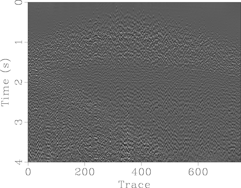
complex1,complexs
Figure 9. Numerically blended synthetic data (complex gather). (a) Unblended data. (b) Blended data. |
|
|


|
|---|
|
complexdeblendedfft1,complexdeblendedslet1,complexdeblendedfxdecon1,complexdifffft1,complexdiffslet1,complexdifffxdecon1,complexerrorfft1,complexerrorslet1,complexerrorfxdecon1
Figure 10. Deblending comparison for numerically blended synthetic data (complex gather). (a) Deblended result using |
|
|

|
|---|
|
complexsnrsa
Figure 11. Diagrams of SNR for synthetic example (complex gather). The "+" line corresponds to seislet-domain thresholding. The "o" line corresponds to |
|
|
|
|
|
|
Iterative deblending of simultaneous-source seismic data using seislet-domain shaping regularization |