Post-stack velocity analysis by separation and imaging of seismic diffractions

Salt detection

gom,gom-dip
Figure 5. Second test example. (a) Near-offset section from a Gulf of Mexico dataset. (b) Local slopes estimated by plane-wave destruction.

gom-pwd,gom-pik
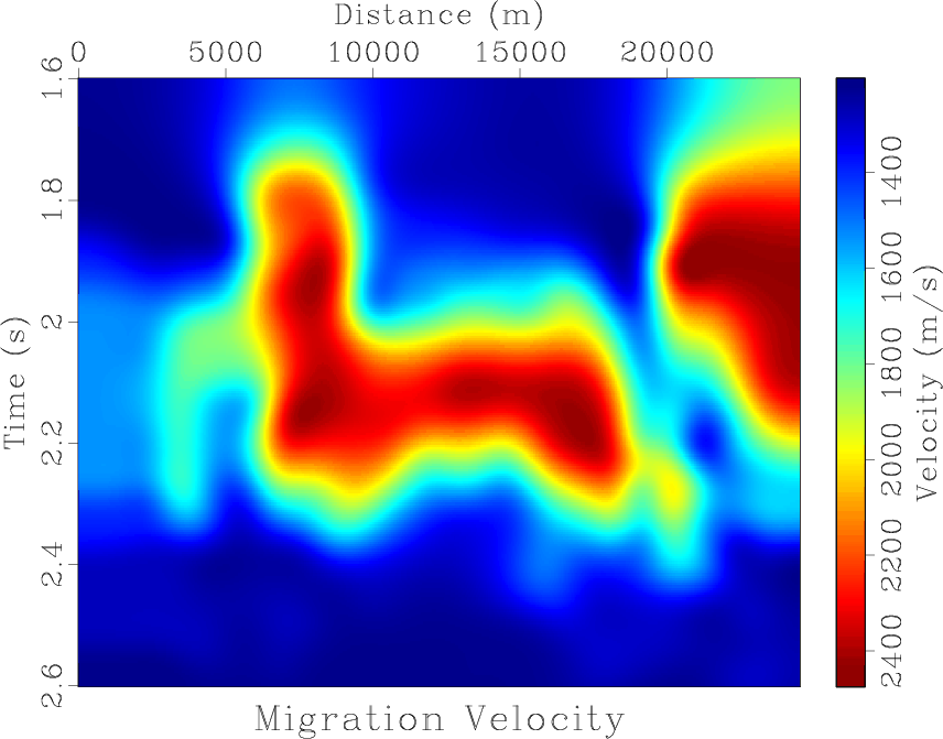
Figure 6. Diffraction separation. (a) Diffraction events separated from data in Figure 5a. (b) Migration velocity picked from local varimax scans after velocity continuation of diffractions.

gom-slc,gom-slc2
Figure 7. Migrated images. (a) Migrated diffractions from Figure 6a. (b) Initial data from Figure 5a migrated with velocity estimated by diffraction imaging.

Figure 5a shows another example, also from the Gulf of Mexico. We used the nearest-offset section for diffraction analysis. Plane-wave destruction estimates dominant slopes of continuous reflection events [Figure 5b] and reveals numerous diffractions generated by rough edges of a salt body [Figure 6a]. We used shaping regularization (Fomel, 2007b) with the smoothing radius of 40-by-10 samples to constrain the slope-estimation process. Focusing analysis generates a time migration velocity [Figure 6b] suitable for collapsing diffractions [Figure 7a]. Both sharp edges of the salt body and continuous specular reflections appear in the final image [Figure 7b]. Inevitably, prestack depth migration (as opposed to time migration) is required to properly position the salt boundary in depth. Time migration, however, provides a reasonable first-order approximation computed at a small fraction of the cost.

Post-stack velocity analysis by separation and imaging of seismic diffractions