|
|
|
|
Dip-separated structural filtering using seislet transform and adaptive empirical mode decomposition based dip filter |
Next: Field data example Up: Example Previous: Example
|
|
|
|
Dip-separated structural filtering using seislet transform and adaptive empirical mode decomposition based dip filter |
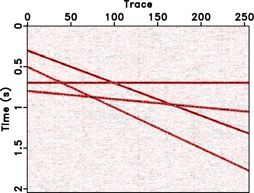
After dip decomposition I remove the crossing points and the local dip conflicts that affect performance of the seislet transform. Figure 7 shows the local slope maps using plane-wave destruction algorithm on separated dip components and original seismic profile.
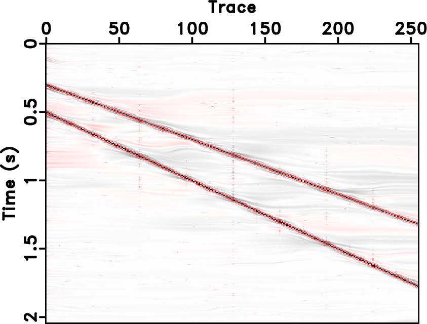
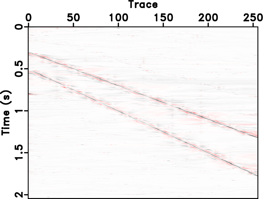
The reconstructed seismic data for each separated dip component after thresholding are shown in Figure 8. Figure 9a is the summation of Figures 8a-8e and thus the output using the proposed approach. Figure 9b is the denoised result using conventional method. In order to demonstrate the superior performance of the proposed over other widely used denoising approaches, I also show the denoised results using the curvelet thresholding approach (Candès et al., 2006a,b) and the ![]() deconvolution method (Canales, 1984). In order to have a fair comparison, I try different parameter combinations in order to obtain the best denoised results with the least loss of useful energy for all the methods. The noise sections corresponding to the proposed approach and the conventional approaches are shown in Figures 10a and 10b. Because of dip conflicts, the seislet domain of the original seismic image is not optimally sparse, and the threshold one use should be more conservative in order to avoid any possible damages to the signals. The resulted denoised image is a bit noisier and the noise section has a lower amplitude level. Although the curvelet transform has directional property, the compactly crossing events make thresholding in the curvelet transform domain not easy to implement, thus one can only use a very conservative threshold value to obtain the optimum denoised result that leaves the least useful energy in the noise section. The noise section using curvelet thresholding is relatively less noisier than other methods, which indicates that more noise are still in the denoised result. The
deconvolution method (Canales, 1984). In order to have a fair comparison, I try different parameter combinations in order to obtain the best denoised results with the least loss of useful energy for all the methods. The noise sections corresponding to the proposed approach and the conventional approaches are shown in Figures 10a and 10b. Because of dip conflicts, the seislet domain of the original seismic image is not optimally sparse, and the threshold one use should be more conservative in order to avoid any possible damages to the signals. The resulted denoised image is a bit noisier and the noise section has a lower amplitude level. Although the curvelet transform has directional property, the compactly crossing events make thresholding in the curvelet transform domain not easy to implement, thus one can only use a very conservative threshold value to obtain the optimum denoised result that leaves the least useful energy in the noise section. The noise section using curvelet thresholding is relatively less noisier than other methods, which indicates that more noise are still in the denoised result. The ![]() deconvolution method can obtain a good denoising performance but might cause some useful dipping energy lost due to the boundary effects. However, using the proposed approach, I obtain an excellent result. The SNR of original noise data is 3.685 dB. The SNR of the denoised data using conventional seislet thresholding is 22.21 dB. The SNRs of the denoised data using the curvelet thresholding and the
deconvolution method can obtain a good denoising performance but might cause some useful dipping energy lost due to the boundary effects. However, using the proposed approach, I obtain an excellent result. The SNR of original noise data is 3.685 dB. The SNR of the denoised data using conventional seislet thresholding is 22.21 dB. The SNRs of the denoised data using the curvelet thresholding and the ![]() deconvolution are 21.07 dB and 20.98 dB, respectively. The SNR of the denoised data using the proposed approach is 24.38 dB. The comparison of SNRs also proves the better performance of the proposed approach than the other approaches. In this example, I preserve 2% coefficients for all the dip components. For the traditional seislet method, I choose a bit more coefficients, 3%, to perform the denoising. For the curvelet method, I choose 6% coefficients to perform the denoising.
deconvolution are 21.07 dB and 20.98 dB, respectively. The SNR of the denoised data using the proposed approach is 24.38 dB. The comparison of SNRs also proves the better performance of the proposed approach than the other approaches. In this example, I preserve 2% coefficients for all the dip components. For the traditional seislet method, I choose a bit more coefficients, 3%, to perform the denoising. For the curvelet method, I choose 6% coefficients to perform the denoising.
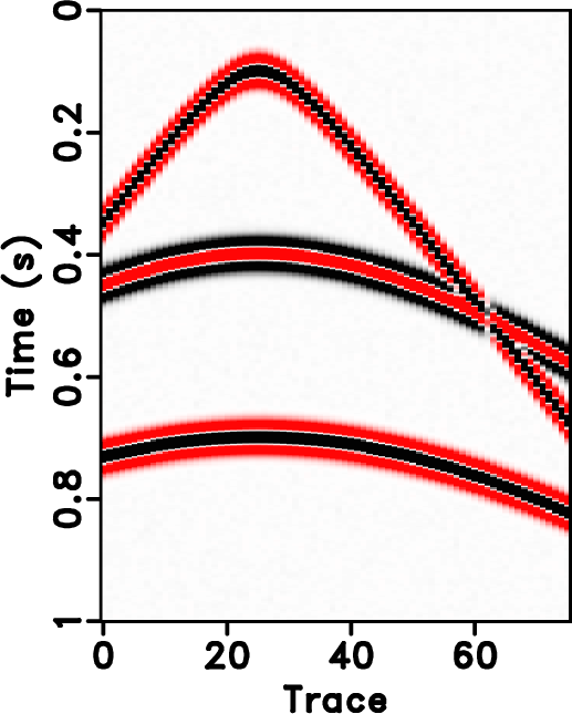
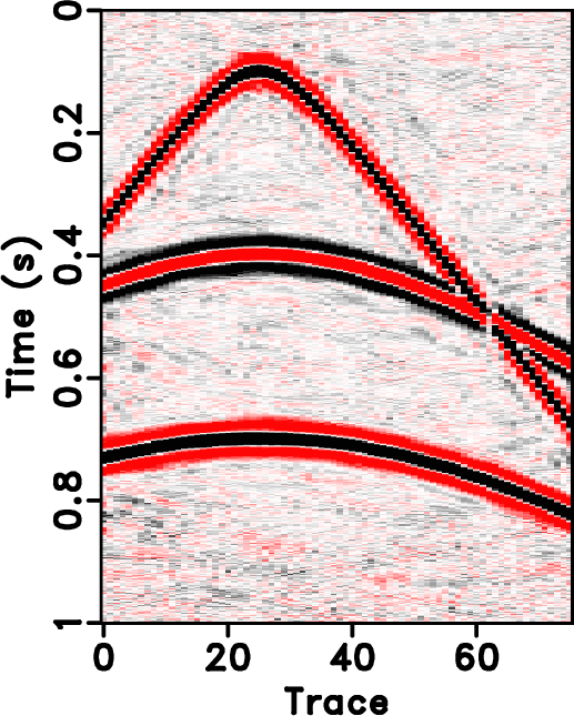
I then use a second synthetic example with curved events to further confirm the superior performance of the proposed approach, as shown in Figures 11 and 12. This example is composed with three curved events with spatially variable slope. The clean and noisy data are shown in Figures 11a and 11d, respectively. Figures 11b, 11c, 11e, and 11f show the denoised performances using the proposed method, traditional seislet method, curvelet method, and ![]() deconvolution method, respectively. Figures 12a, 12b, 12c, and 12d show their corresponding removed noise sections. It is obvious that the proposed approach can obtain the cleanest denoised data while the other three methods cause a bit more random noise left in the denoised images. The SNR improvements using four different approaches are 10.18 dB, 9.54 dB, 9.27 dB, and 7.98 dB, respectively. In this example, I preserve 3% coefficients for all the dip components, preserve 5 % coefficients for the traditional seislet method, and 8% for the curvelet method.
deconvolution method, respectively. Figures 12a, 12b, 12c, and 12d show their corresponding removed noise sections. It is obvious that the proposed approach can obtain the cleanest denoised data while the other three methods cause a bit more random noise left in the denoised images. The SNR improvements using four different approaches are 10.18 dB, 9.54 dB, 9.27 dB, and 7.98 dB, respectively. In this example, I preserve 3% coefficients for all the dip components, preserve 5 % coefficients for the traditional seislet method, and 8% for the curvelet method.


|
|---|
|
plane-c,plane
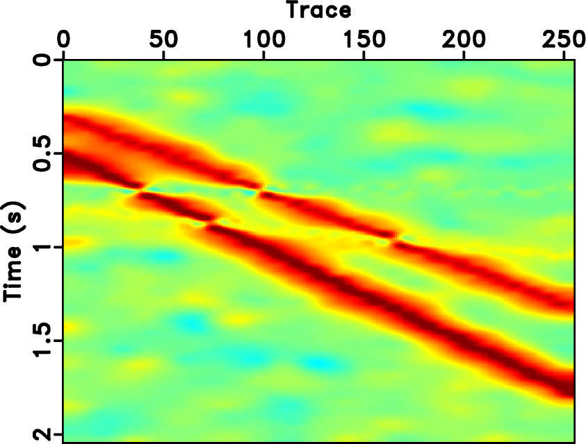
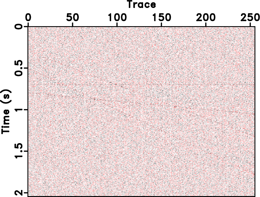
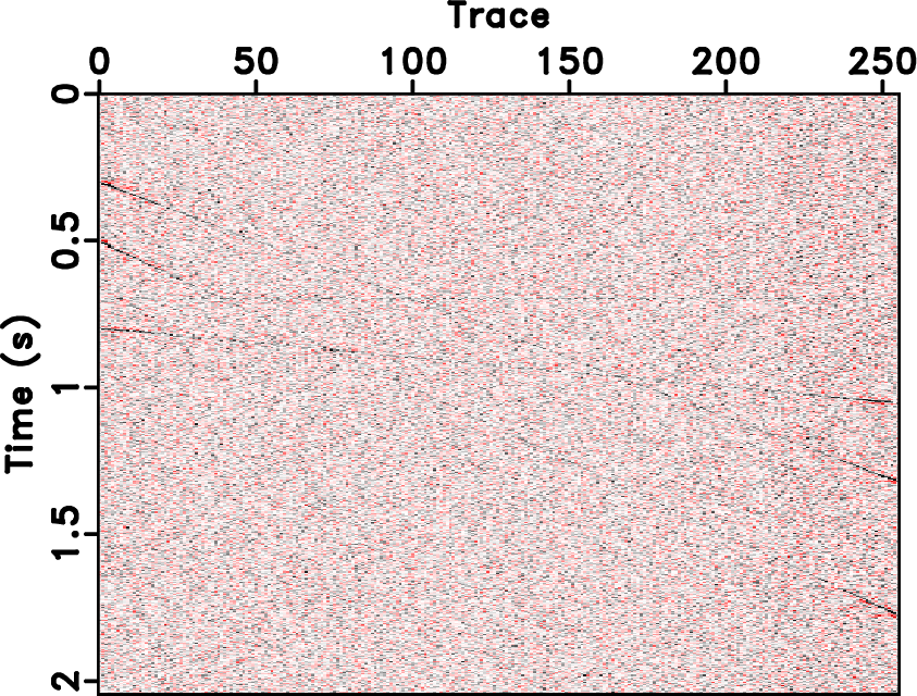
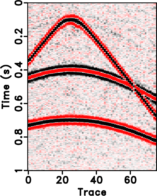
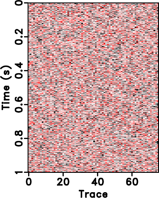
Figure 5. First synthetic example. (a) Clean data. (b) Noisy data. |
|
|


|
|---|
|
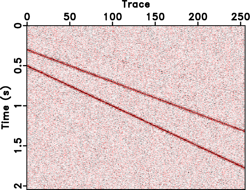
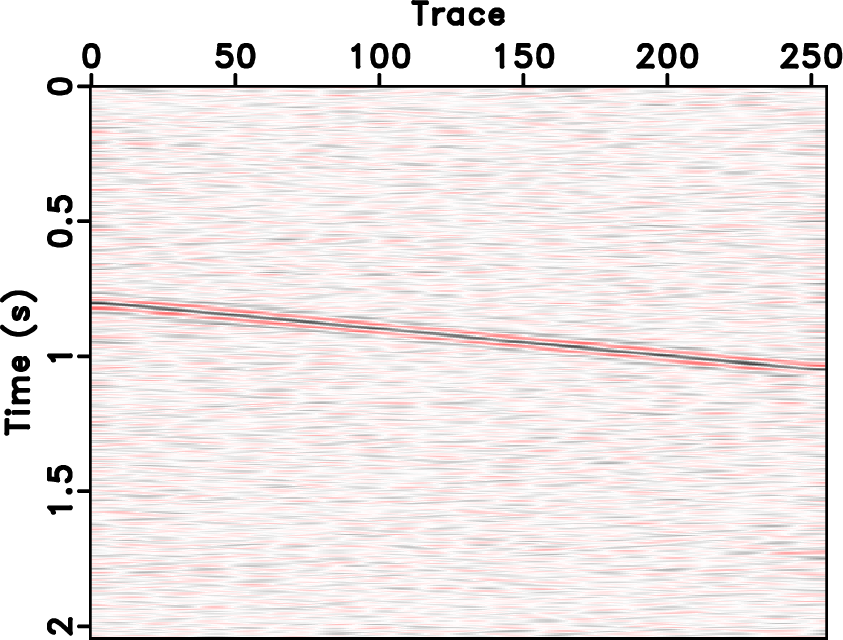
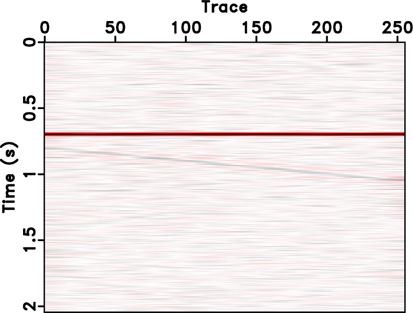
dip1,dip2,dip3,dip4,dip5
Figure 6. Separated dip components using EMD based dip filter for synthetic data. (a) First dip component. (b) Second dip component. (c) Third dip component. (d) Fourth dip component. (e) Last dip component. |
|
|


|
|---|
|
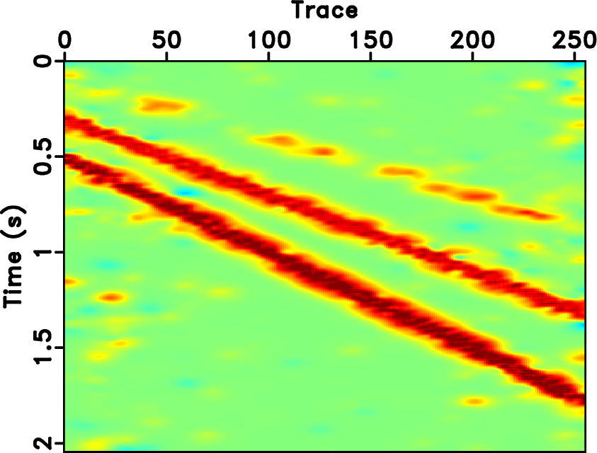
dip1-emd-p,dip2-emd-p,dip3-emd-p,dip4-emd-p,dip5-emd-p,plane-dip
Figure 7. Local slope comparison for synthetic data. (a) First local slope map. (b) Second local slope map. (c) Third local slope map. (d) Fourth local slope map. (e) Fifth local slope map. (f) Local slope map before dip separation. |
|
|


|
|---|
|
dip1-emd0,dip2-emd0,dip3-emd0,dip4-emd0,dip5-emd0
Figure 8. (a) Denoised first dip component. (b) Denoised second dip component. (c) Denoised third dip component. (d) Denoised fourth dip component. (e) Denoised fifth dip component. |
|
|


|
|---|
|
plane-emdseis,plane-recon,plane-curv,plane-fx
Figure 9. Denoised results for the first synthetic data. (a) Denoised result using the proposed method (summation of (a)-(e) in Figure 8). (b) Denoised result using the conventional seislet thresholding method. (c) Denoised result using the curvelet thresholding method. (d) Denoised result using the |
|
|


|
|---|
|
plane-emdseis-dif,plane-seis-dif,plane-curv-dif,plane-fx-dif
Figure 10. Denoised results for the first synthetic data. (a) Denoised result using the proposed method (summation of (a)-(e) in Figure 8). (b) Denoised result using the conventional seislet thresholding method. (c) Denoised result using the curvelet thresholding method. (d) Denoised result using the |
|
|


|
|---|
|
hyper-c,hyper-e,hyper-s-0,hyper,hyper-ct-0,hyper-fx-0
Figure 11. Second synthetic example. (a) Clean data. (b) Denoised data using the proposed approach. (c) Denoised data using the traditional seislet thresholding approach. (d) Noisy data. (e) Denoised data using the curvelet transform. (f) Denoised data using |
|
|


|
|---|
|
hyper-e-n,hyper-s-n-0,hyper-ct-n-0,hyper-fx-n-0
Figure 12. Removed noise sections for the second synthetic example. (a) Noise section using the proposed method. (b) Noise section using the conventional seislet thresholding method. (c) Noise section using the curvelet thresholding approach. (d) Noise section using |
|
|
|
|
|
|
Dip-separated structural filtering using seislet transform and adaptive empirical mode decomposition based dip filter |