Kirchhoff migration using eikonal-based computation of traveltime source-derivatives

Acknowledgments

We thank the editors, Samuel Gray, and three anonymous reviewers for constructive suggestions that helped improving the quality of the manuscript. We thank Tariq Alkhalifah and Alexander Vladimirsky for useful discussions and sponsors of the Texas Consortium for Computational Seismology (TCCS) for financial support of this research. This publication is authorized by the Director, Bureau of Economic Geology, The University of Texas at Austin.

Appendix A

FMM implementation of source-derivatives

The FMM is a non-iterative eikonal solver with $O(N \log N)$ complexity, where $N$ is the total number of grid points of the discretized domain. It relies on a heap data structure to keep the updating sequence, and a local one-sided upwind finite-difference scheme for ensuring the causality (Sethian, 1996). Consider in 3D a cubic domain discretized into Cartesian grids, with uniform grid size of $(\Delta x,\Delta y,\Delta z)$. 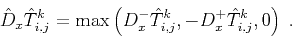Let $\hat{T}_{i,j}^k$ be the traveltime value at vertices $\mathbf{x}_{i,j}^k = (x_i,y_j,z_k)$ and define difference operator $D_x^{\pm}$ for $x$ direction as

$$D_x^{\pm} \hat{T}_{i,j}^k = \pm \frac{\hat{T}_{i \pm 1,j}^k - \hat{T}_{i,j}^k}{\Delta x}\;,$$ (14)

The causality condition requires picking an upwind neighbor in all directions at $\mathbf{x}_{i,j}^k$.

$$\hat{D}_x \hat{T}_{i,j}^k = \max \left( D_x^- \hat{T}_{i,j}^k, -D_x^+ \hat{T}_{i,j}^k, 0 \right)\;.$$ (15)

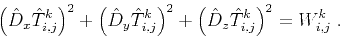
After similar definitions for $\hat{D}_y$ and $\hat{D}_z$, the local upwind scheme in FMM for equation 3 reads

$$\left( \hat{D}_x \hat{T}_{i,j}^k \right)^2 + \left( \hat{D}_... ...^2 + \left( \hat{D}_z \hat{T}_{i,j}^k \right)^2 = W_{i,j}^k\;.$$ (16)

For $\partial \hat{T} / \partial \mathbf{x}$ in equation 6 and $\partial \hat{T} / \partial \mathbf{q}$ in equation 5, we can apply the same upwind strategy:

$$\hat{D}_x \hat{T}_{i,j}^k \cdot \hat{D}_x \left( \frac{\par... ...eft( \frac{\partial W}{\partial \mathbf{x}} \right)_{i,j}^k\;,$$ (17)

$$\left( \frac{\partial \hat{T}}{\partial \mathbf{q}} \right)_... ...\hat{D}_\mathbf{q} \hat{T}_{i,j}^k,\,\,\mathbf{q} = (x,y,z)\;.$$ (18)

where in equation A-4 $\hat{D}_x$, $\hat{D}_y$ and $\hat{D}_z$ are chosen according to $\hat{T}_{i,j}^k$, regardless of $\partial \hat{T} / \partial \mathbf{x}$. Finally,

$$\left( \frac{\partial T}{\partial \mathbf{x_s}} \right)_{i,j... ...frac{\partial \hat{T}}{\partial \mathbf{q}} \right)_{i,j}^k\;.$$ (19)

To incorporate the computation of traveltime source-derivatives into FMM, one only needs to add equations A-4, A-5 and A-6 after A-3. An extra upwind sorting and solving after pre-computing $\hat{T}$ is not necessary. The total complexity of FMM with the auxiliary output of traveltime source-derivative remains $O(N \log N)$.

Appendix B

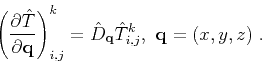
Interpolation of source-derivatives

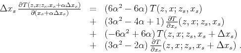
Applying the chain-rule 13 to equation 10, we arrive at the interpolation equation for source-derivatives in the cubic Hermite scheme:

$$\begin{array}{lcl} \Delta x_s\, \frac{\partial T (z,x; z_s,x... ...ial T}{\partial x_s} (z,x; z_s,x_s + \Delta x_s)\;. \end{array}$$ (20)

Analogously, the interpolation of source-derivatives in the linear scheme 11 reads:

$$\begin{array}{lcl} \Delta x_s\, \frac{\partial T (z,x; z_s,x... ...T (z,x; z_s,x_s) + T (z,x; z_s,x_s + \Delta x_s)\;. \end{array}$$ (21)

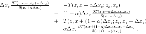
which is a simple first-order finite-difference estimation. Finally, in the case of shift scheme 12, the partial derivative $\partial / \partial \alpha$ must be applied to the shifted traveltime terms at the same time:

$$\begin{array}{lcl} \Delta x_s\, \frac{\partial T (z,x; z_s,x... ...Delta x_s)} {\partial (x+(1-\alpha) \Delta x_s)}\;. \end{array}$$ (22)

The required spatial derivatives can be estimated from the traveltime table by means of finite-differences, for example by using the upwind approximation A-2.

Kirchhoff migration using eikonal-based computation of traveltime source-derivatives