|
|
|
|
On anelliptic approximations for |
Similar strategy is applicable for approximating the group velocity. Applying the shifted hyperbola approach to ``unlinearize'' Muir's approximation (17), we seek an approximation of the form
Although there is no simple explicit expression for the transversally
isotropic group velocity, we can differentiate the parametric representations
of ![]() and
and ![]() in terms of the phase angle
in terms of the phase angle ![]() that follow from
equation (5). The group velocity is an even function of the angle
that follow from
equation (5). The group velocity is an even function of the angle
![]() because of the VTI symmetry. Therefore, the odd-order derivatives are
zero at the axis of symmetry (
because of the VTI symmetry. Therefore, the odd-order derivatives are
zero at the axis of symmetry (
![]() ). Fitting the second-order
derivative
). Fitting the second-order
derivative
![]() at
at ![]() produces
produces
![]() ,
consistent with Muir's approximation (17). Fitting additionally
the fourth-order derivative
,
consistent with Muir's approximation (17). Fitting additionally
the fourth-order derivative
![]() at
at ![]() produces
produces
The final group velocity approximation takes the form
Approximation (33) turns out to be remarkably accurate for this example. It appears nearly exact for group angles up to 45 degrees from vertical and does not exceed 0.3% relative error even at larger angles. It is compared with two other approximations in Figure 5. These are the Zhang-Uren approximation (Zhang and Uren, 2001) and the Alkhalifah-Tsvankin approximation, which follows directly from the normal moveout equation suggested by Alkhalifah and Tsvankin (1995):
Another accurate group velocity approximation was suggested by Alkhalifah (2000b). However, the analytical expression is complicated and inconvenient for practical use. The accuracy of Alkhalifah's approximation for the Greenhorn shale example is depicted in Figure 6.

|
|---|
|
errgrp
Figure 4. Relative error of different group velocity approximations for the Greenhorn shale anisotropy. Short dash: Thomsen's weak anisotropy approximation. Long dash: Muir's approximation. Solid line: suggested approximation. |
|
|

|
|---|
|
errgrp2
Figure 5. Relative error of different group velocity approximations for the Greenhorn shale anisotropy. Short dash: Alkhalifah-Tsvankin approximation. Long dash: Zhang-Uren approximation. Solid line: suggested approximation. |
|
|

|
|---|
|
errgrp4
Figure 6. Relative error of different group velocity approximations for the Greenhorn shale anisotropy. Dashed line: Alkhalifah approximation. Solid line: suggested approximation. |
|
|
It is similarly possible to convert a group velocity approximation into the
corresponding moveout equation. In a homogeneous anisotropic medium, the
reflection traveltime ![]() as a function of offset
as a function of offset ![]() is
is
Figure 7 compares the accuracy of different moveout approximations assuming reflection from the bottom of a homogeneous anisotropic layer of 1 km thickness with the elastic parameters of Greenhorn shale. Approximation (39) appears extremely accurate for half-offsets up to 1 km and does not develop errors greater than 5 ms even at much larger offsets.

|
|---|
|
timepp
Figure 7. Traveltime moveout error of different group velocity approximations for Greenhorn shale anisotropy. The reflector depth is 1 km. Short dash: Alkhalifah-Tsvankin approximation. Long dash: Zhang-Uren approximation. Solid line: suggested approximation. |
|
|
It remains to be seen if the suggested approximation proves to be useful for describing normal moveout in layered media. The next section discusses its application for traveltime computation in heterogenous velocity models.
|
|
|
|
On anelliptic approximations for |
![$\displaystyle S = \frac{1}{2}\,\frac{ \left[(l+f)^2 + l\,(c-l)\right]^2\,\left[...
... - (l+f)^2\right]}{ a^2\,c\,(c-l)\,(l+f)^2 - \left[l\,(c-l) + (l+f)^2\right]^3}$](img107.png)

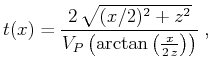
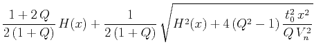
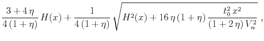
![$\displaystyle t^2(x) \approx t_0^2 + \frac{x^2}{V_n^2} - \frac{2\,\eta\,x^4}{V_n^2\,\left[t_0^2\,V_n^2 + (1+ 2\,\eta)\,x^2\right]} \;,$](img116.png)
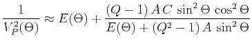
![$\displaystyle \frac{1}{V_P^2(\Theta)} \approx \frac{\cos^2{\Theta}}{V_z^2} + \f...
...2\,\left[\cos^2{\Theta}\,V_n^2/V_z^2 + (1+ 2\,\eta)\,\sin^2{\Theta}\right]} \;,$](img120.png)