|
|
|
|
Matching and merging high-resolution and legacy seismic images |


|
|---|
|
window1,window2
Figure 8. The first 600 ms of data from a sample line from the legacy, high-resolution, and merged image (a). The same images with depth for the legacy, high-resolution, and merged images (b). The merged image resembles the high-resolution image in the shallow parts and incorporates the more coherent lower frequency information from the legacy image with depth. |
|
|
Due to the nature of acquisition, the high resolution image has very dense spatial coverage, providing detailed time slices of the near subsurface (Meckel and Mulcahy, 2016). The legacy image has lower spatial resolution. As a result, when matching the high-resolution and legacy images spatially, the high spatial resolution of the high-resolution image must be degraded to match that of the legacy image. We rebinned the legacy and high-resolution images to align them spatially for comparison (Figure 10). We chose to spatially down-sample the high-resolution image to match the legacy image as opposed to interpolating the legacy image to the high-resolution image's spatial grid to prevent potentially introducing inaccurate data in the merged image.
There is a definite separation in frequency content when comparing the legacy and high-resolution images (Figure 9). Because there is not much overlap in frequency bandwidth, balancing their spectral content is challenging. In addition, a primary assumption made in deriving the theoretical smoothing radius (equation 6) is that the signal is modeled by a summation of Ricker wavelets, which may not be a correct assumption. As a result, additional steps must be taken beyond applying the smoothing specified by equation (6) to ensure matching frequency content.
We first apply a low-cut filter to the legacy data to remove the low frequency information that is simply not present in the high-resolution image. Next, we adjust the non-stationary smoothing radius using a simple iterative algorithm (Greer and Fomel, 2017).
The main premise behind the algorithm comes from the fact that, in general, the greater the smoothing radius at a specified point, the more high frequencies are attenuated by smoothing. We choose an initial guess of the non-stationary smoothing radius before applying corrections based on two primary assumptions:
We apply these assumptions using a line-search method:
Using this method, we can continually adjust the smoothing radius until we achieve the desired result of balancing the local frequency content between the two images. In practice, this method produces an acceptable solution in approximately 5 iterations and exhibits sublinear convergence. We smooth the high-resolution image with the radius this method produces to balance local frequency content between the two images.
After this, we use the low-cut filtered legacy and smoothed high-resolution images to find estimated time shifts we need to apply to the high-resolution image to align the reflections with the legacy image. Then, we apply this estimated time shift to the original high-resolution image and blend it with the original legacy image as specified by equations (7) and (9).
The resultant merged image is shown in Figure 10c. The frequency content of the merged image is shown in Figure 9. Here, the merged image spans the frequency bandwidth of the two initial images, thus producing a high resolution volume including optimal signal characteristics from the two initial images.

|
|---|
|
nspectra2
Figure 9. The spectral content of the entire image display of the legacy (red dashed), high-resolution (blue dotted), and resultant merged (magenta solid) images for the second data set. |
|
|


|
|---|
|
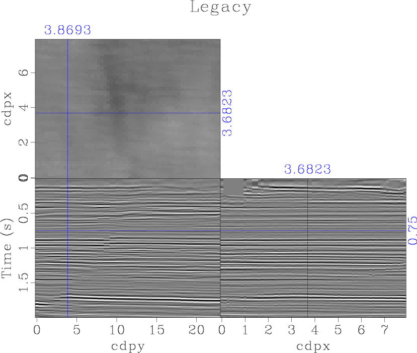
legacy4,hires4,merge3
Figure 10. The legacy (a), high-resolution (b), and resultant merged (c) images of the second data set. |
|
|
|
|
|
|
Matching and merging high-resolution and legacy seismic images |
![\begin{displaymath}
\mathbf{r} = \mathbf{F}[\mathbf{S}_{\mathbf{R}} \mathbf{d}_h] - \mathbf{F}[\mathbf{d}_l]\;,
\end{displaymath}](img36.png)