|
|
|
|
Random noise attenuation using local signal-and-noise orthogonalization |

|
|---|
|
demo
Figure 12. Demonstration of signal-and-noise orthogonalization. |
|
|
As shown schematically in Figure A-1, the initially estimated signal and noise are denoted by
![]() and
and
![]() , respectively. By projecting
, respectively. By projecting
![]() to the direction of
to the direction of
![]() , we can get the projection
, we can get the projection
![]() . The other component of
. The other component of
![]() is the final estimated noise, as shown in equation 3. The final estimated signal is thus the summation of the initially estimated signal
is the final estimated noise, as shown in equation 3. The final estimated signal is thus the summation of the initially estimated signal
![]() and the projection component
and the projection component
![]() .
.
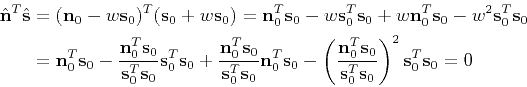
When
 , the following equation holds:
|
|
|
|
Random noise attenuation using local signal-and-noise orthogonalization |