Ground-roll noise attenuation using a simple and effective approach based on local bandlimited orthogonalization

Local signal-and-noise orthogonalization

The principle of our technique is to locally orthogonalize the denoised signal and noise sections in order to ensure no coherent primary reflections will be lost in the noise section. Here, we propose to apply the algorithm to the ground-roll noise removal problem. The orthogonalization based approach can be summarized as:

$$\mathbf{s} =(\mathbf{I}+\mathbf{W})\mathbf{\hat{d}},$$ (2)

$$\mathbf{n} =\mathbf{\hat{d}}-(\mathbf{I}+\mathbf{W})\mathbf{\hat{d}}.$$ (3)

Here, $\mathbf{s}$ and $\mathbf{n}$ are the output denoised signal and noise sections. $\mathbf{I}$ denotes an identity matrix. $\mathbf{W}$ denotes a diagonal operator composed of the local orthogonalization weight (LOW) vector. When $w=\frac{\mathbf{n}_0^T\mathbf{s}_0}{\mathbf{s}_0^T\mathbf{s}_0}$ , $\mathbf{s}_0$ and $\mathbf{n}_0$ denoting the initial guess of signal and noise, $w$ is the global orthogonalization weight (GOW), it can be proved 7 that the following scaled signal $\mathbf{s}_0$ and corresponding noise $\mathbf{n}_0$ are orthogonal to each other in a global sense:

$$\hat{\mathbf{n}} = \mathbf{n}_0 - w\mathbf{s}_0,$$ (4)

$$\hat{\mathbf{s}} = \mathbf{s}_0 + w\mathbf{s}_0.$$ (5)

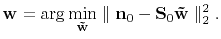
In a local sense, the LOW can be define as:

$$w_m(t) = \frac{\displaystyle\sum_{i=t-m/2}^{t+m/2} s_0(i) n_0(i)}{\displaystyle\sum_{i=t-m/2}^{t+m/2} s_0^2(i)},$$ (6)

where $w_m(t)$ denotes the LOW for each temporal point $t$ with a local window length $m$ . $s_0(t)$ and $n_0(t)$ here denote the initially estimated signal and noise for each point $t$ .

In order to better control the locality and smoothness of LOW, we follow the local-attribute scheme introduced by Fomel (2007a):

$$\mathbf{w} = \arg\min_{\mathbf{\tilde{w}}} \parallel \mathbf{n}_0 - \mathbf{S}_0\mathbf{\tilde{w}}\parallel_2^2. %+ \mathbf{R}(\mathbf{w})$$ (7)

Here, $\mathbf{w}$ is the LOW, $\mathbf{S}_0$ is a diagonal matrix composed of the initial estimated signal $\mathbf{s}_0$ : $\mathbf{S}_0=diag(\mathbf{s}_0)$ . Then, we solve the least-squares problem 7 with the help of shaping regularization (a novel regularization framework for obtaining a faster convergence and a better control on the model behavior, originated from the seismic data processing community Fomel (2007b)) using a local-smoothness constraint:

$$\mathbf{w} = [\lambda^2\mathbf{I} + \mathcal{T}(\mathbf{S}_0^T\mathbf{S}_0-\lambda^2\mathbf{I})]^{-1}\mathcal{T}\mathbf{S}_0^T\mathbf{n}_0,$$ (8)

where $\mathcal{T}$ is a triangle smoothing operator and $\lambda$ is a scaling parameter set as $\lambda = \Arrowvert\mathbf{S}_0^T\mathbf{S}_0\Arrowvert_2$ Fomel (2007a). The triangle smoothing operator was introduced in detail in Fomel (2007b). It should be mentioned that solution of equation 7 corresponds to a regularized division (an element-wise division between two vectors can be treated as an inverse problem with some constraints in order to ensure the stability) between the two vectors $\mathbf{n}_0$ and $\mathbf{s}_0$ and it can be solved using any regularization approach, not limited to the shaping regularization strategy shown in equation 8. Thus it is fairly convenient to implement the local orthogonalization between initial signal and noise. A more detailed mathematical description about the local orthogonalization methodology can be found in Chen and Fomel (2015) and a demonstration about the physical meaning of orthogonalization can be found in the Appendix A in Chen and Fomel (2015).

Ground-roll noise attenuation using a simple and effective approach based on local bandlimited orthogonalization