Toy Model Example

Next: Synthetic Example Up: Examples Previous: Examples

Toy Model Example

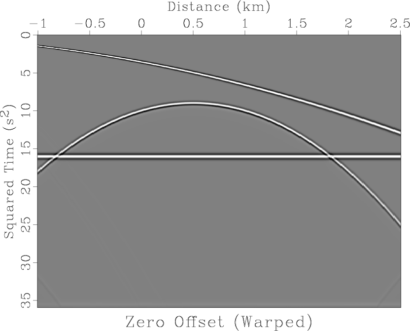
We first illustrate the concept of oriented velocity continuation using a simple toy model (Landa et al., 2008; Klokov and Fomel, 2013) with constant $\frac{km}{s}$ velocity containing one dipping and one flat reflector and a single diffractor centered at 0.5 km (Figure 1a). Figure 1b shows data warped to squared time.

Warped data are decomposed into their constituent slope components and initially under-migrated using $v_0=0.5 \frac{km}{s}$ . The initial slope decomposed image is shown in Figure 2, which illustrates a slope gather centered above the diffractor on the right panel, and a partial image containing energy with the slope of the top dipping reflector on the front panel. The partial image contains energy of the top dipping reflector, which has the selected slope, diffraction energy with that slope, and a small portion of the energy from the flat bottom reflector. Stacking over all constituent slopes provides an image (top left panel of Figure 4).

The slope decomposed initial migration from Figure 2 is propagated through a suite of plausible migration velocities. We illustrate the initial migration and example velocities of $\frac{km}{s}$ , $\frac{km}{s}$ (the correct velocity), and $\frac{km}{s}$ . Slope gathers showing this process are shown in Figure 3. Stacking these propagated images over slope produces the image in Figure 4.


data,data2 Figure 1. Toy model data: (a) zero-offset synthetic data featuring two sloping reflectors and a diffractor centered at ; (b) zero-offset data warped to squared time.


ovc0 Figure 2. Slope decomposed initial migration for toy model data using $v_0=0.5 \frac{km}{s}$ . The side pane shows the slope decomposed data centered at , the diffractor, and the front pane shows a partial image for data containing energy with a slope of $2.998 \frac{km}{s^2}$ , that of the top reflector.

Examining the slope gather of the initial migration in Figure 3a, the three panels contain points of energy corresponding, from top to bottom, to the top reflector, the diffractor, and the bottom reflector. The energy of each reflector is contained at the same lateral position in the three panels due to the constant slope of the reflector, although the vertical position of the top dipping reflector changes through the panels because the reflector dips downward to the right.

The diffraction has a hyperbolic moveout rather than a constant slope, so energy appears at different slopes in different slope gathers, with zero slope in the gather centered over the diffractor at 0.5 km. As we propagate data through velocity, this pattern holds: the reflection energy is stationary at its slope location for all gathers and diffraction energy has zero slope when viewed in the gather above the diffractor and non-zero slope for other gathers.

The initially migrated image is propagated to the higher time migration velocity of $0.75 \frac{km}{s}$ using oriented velocity continuation, and slope gathers are illustrated in Figure 3b. Reflection energy now bends upward about the stationary point of each reflection in ``smiles" that become more accentuated with larger migration velocities. The diffraction event bends upward as well, but this only holds for the current case of under-migration.

Figure 3c shows the image propagated to the correct migration velocity. Diffraction energy is planar in all three gathers and flat in the middle gather centered above the diffractor. Stacking the energy in each gather over slope collapses the flat diffraction energy in the central gather to a point at the location of the diffractor. Sloping diffraction energy in the right and left panels cancels out when summed over slope. This flatness is essential to using oriented velocity continuation as a tool for determining the correct migration velocity.

When data are further propagated to over-migration with velocity of $\frac{km}{s}$ in Figure 3d, the diffraction event bows downward in a ``frown" juxtaposed against the upward bending reflection ``smiles".

Stacking over slope provides images for these four velocities (Figure 4). In these images, the diffraction event incrementally evolves from having a hyperbolic downward character in the top under-migrated row, to collapsing to a point in the bottom left panel with the correct migration velocity, to bowing hyperbolically upward in the bottom right over-migrated image.

The changing geometry of diffraction energy in the gathers can be harnessed to determine the proper migration velocity (Landa et al., 2008; Reshef and Landa, 2009). The correct migration velocity will be the one that maximizes the ``flatness" of slope decomposed diffraction events, as measured by coherence or another appropriate metric. Selecting $\frac{km}{s}$ , the velocity that produces flat diffraction energy, provides us with a properly migrated image (Figure 5).

To properly estimate migration velocity using diffraction flatness, reflection events must first be filtered out from the diffraction data, or else the contribution of reflection ``smiles" may dominate and bias the flatness measure.


cig0,cig1,cig2,cig3 Figure 3. Slope gathers centered at (left), (center), and (right) for migration velocities of: (a) initial under-migration with $0.5 \frac{km}{s}$ ; (b) under-migration with $0.75 \frac{km}{s}$ ; (c) the correct migration velocity of $1.0 \frac{km}{s}$ ; (d) over-migration with $1.25 \frac{km}{s}$ .