|
|
|
|
Local skewness attribute as a seismic phase detector |
The method of local attributes (Fomel, 2007a) is a technique for
extending stationary or instantaneous attributes to smoothly varying
or nonstationary attributes by employing a regularized least-squares
formulation. In particular, the scalar
correlation coefficient ![]() in equation 2 is replaced
with a vector,
in equation 2 is replaced
with a vector, ![]() , defined
as a componentwise product of vectors
, defined
as a componentwise product of vectors ![]() and
and
![]() , where
, where
Regularized inversion appearing in equations 7 and 8 is justified in the method of shaping regularization (Fomel, 2007b). The corresponding local similarity attribute has been used previously to align multicomponent and time-lapse images (Kazemeini et al., 2010; Zhang et al., 2013; Fomel, 2007a; Fomel and Jin, 2009), to detect focusing of diffractions (Fomel et al., 2007), to enhance stacking (Liu et al., 2009,2011a), to create time-frequency distributions (Liu et al., 2011b), and to perform zero-phase correction with local kurtosis (Van der Baan and Fomel, 2009). In this paper, we apply it to zero-phasing seismic data using local skewness.


|
|---|
|
trace,tskew,trace0
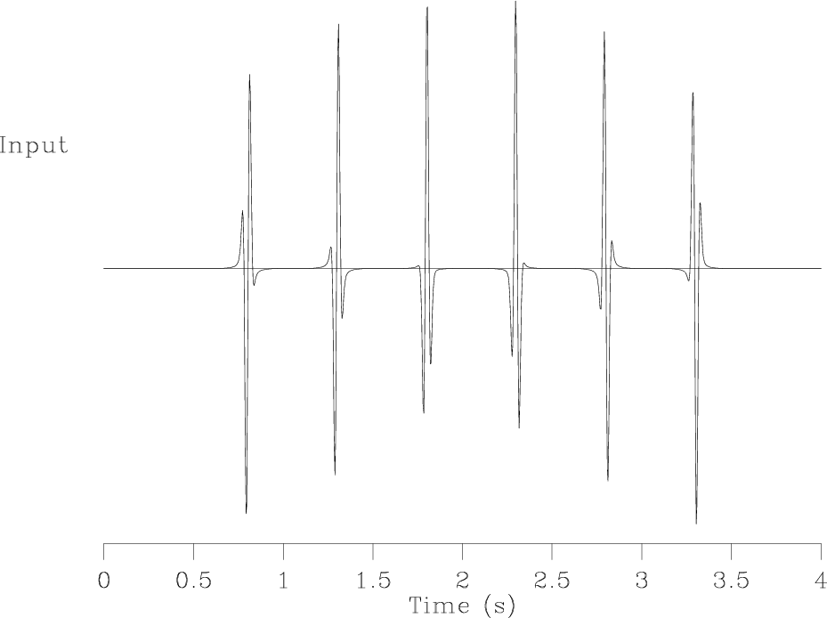
Figure 5. (a) Input synthetic trace with variable-phase events. (b) Inverse local skewness as a function of the phase rotation angle. Red colors correspond to high inverse similarity. (c) Synthetic trace after non-stationary rotation to zero phase using picked phase. |
|
|
We illustrate the proposed zero-phase correction procedure in
Figure 5. The input synthetic trace
contains a set of Ricker wavelets with a gradually variable phase
(Figure 5a). We start with a number of phase rotations
with different angles, each time computing the local skewness. The
result of this step is displayed in Figure 5b and shows a
clear high-similarity trend. After picking the trend, adding
![]() to it, and performing the corresponding nonstationary
trace rotation, we end up with the phase-corrected trace, shown in
Figure 5c. All the original phase rotations are clearly
detected and removed. The radius of the
regularization smoothing in this example was 100 samples or 0.4 s.
to it, and performing the corresponding nonstationary
trace rotation, we end up with the phase-corrected trace, shown in
Figure 5c. All the original phase rotations are clearly
detected and removed. The radius of the
regularization smoothing in this example was 100 samples or 0.4 s.
|
|
|
|
Local skewness attribute as a seismic phase detector |
![$\displaystyle \left[\lambda^2 \mathbf{I} +
\mathbf{S} \left(\mathbf{A}^T \...
...bda^2 \mathbf{I}\right)\right]^{-1}
\mathbf{S} \mathbf{A}^T \mathbf{b}\;,$](img31.png)
![$\displaystyle \left[\lambda^2 \mathbf{I} +
\mathbf{S} \left(\mathbf{B}^T \...
...bda^2 \mathbf{I}\right)\right]^{-1}
\mathbf{S} \mathbf{B}^T \mathbf{a}\;.$](img33.png)