|
|
|
|
A reversible transform for seismic data processing |
Now that the general form of the transform has been developed, an appropriate method is needed to implement it. The method we review and discuss here is matrix vector multiplication.
In order to computationally implement an integral transform, recognize that the input function can be viewed as a vector, or a one-dimensional array, and that the transform kernel can be viewed as a matrix, or a two-dimensional array. The output of a matrix vector multiplication is analogous to the output function of the integral, but it is another vector along a new coordinate axis. The important feature of matrix vector multiplication is that it can be used to simultaneously multiply and integrate two functions over an input index. This concept is certainly not new to engineering or geophysics, and many of its benefits have been explored in detail (Claerbout, 1992).
Constructing a matrix operator for the forward and inverse data processing transform follows the same procedure one would use for any transform operator. The general procedure is summarized here:
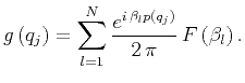
The concise form of the forward data processing transform can be cast as a matrix vector multiplication following the above steps as:
The inverse data processing transform is more similar in form to the forward Fourier transform, in that it takes the series from the input domain and outputs a Fourier spectrum. Again following the procedure to construct a transform matrix, we cast the inverse data processing transform (11) as a matrix-vector multiplication:
Although not necessary for implementation, it is insightful to separate the data processing transform matrices as a composition of a Fourier transform matrix with a shifting matrix.
For a set of traces that are of the same length, the only part of the data processing transform matrix that changes from trace to trace is the shifting exponential.
It is only because of the unique form of the shift itself that the exponentials reduce to a single transform exponential.
Before this reduction, the Fourier transform matrices can be constructed separately from the forward and reverse shifting matrices for the same data.
The construction of the Fourier transform matrices is well-known, and elements of the forward shift matrix,
![]() , are given by:
, are given by:
The inverse of the discrete data processing transform can be exactly formulated as in the continuous case.
The discrete data processing transform has very similar form to the Fourier matrices, and its approximate inverse is easily calculated.
From equations 18 and 19, we claim that the inverse matrix for each trace can be accurately approximated by the adjoint of the forward matrix, scaled by
![]() .
.
|
|
|
|
A reversible transform for seismic data processing |
![$\displaystyle F \left( \beta _l \right) = \sum _{l=1}^N \frac{\left[ \alpha \le...
..., \beta_j \, p \left( q_l \right)} \right]}{2 \, \pi} \, f \left( p_l \right) ,$](img62.png)