A fast algorithm for 3D azimuthally anisotropic velocity scan

Example 1

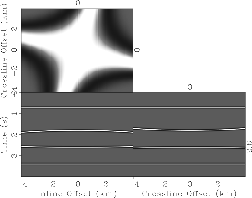
We first consider a simple 3D synthetic CMP gather consisting of four isolated events, each with a different degree of azimuthal anisotropy (Figure 2a). The moveout parameters $\tau$ , $W_{\text{avg}}$ , $W_{\cos}$ , and $W_{\sin}$ used to generate the events are specified in Table 1. Figure 2b shows the data after isotropic NMO using the exact $W_{\text{avg}}$ . Except for the first flattened isotropic event, the other three events clearly require an additional moveout. The computed semblance by the fast algorithm is shown in Figure 3, where manually picked parameters coincide well with exact values. Besides accuracy, what is remarkable is that, even for this moderate-sized problem ( $N_t=N_{\tau}=1000$ , $N_x=N_y=N_{W_{\cos}}=N_{W_{\sin}}=100$ ), CPU time of the butterfly algorithm (for a single Radon transform) is about 139 s, whereas the direct velocity scan takes 4681 s.

Table 1: Parameters used to generate the seismic events in Figure 2.

event	$\tau$	$W_{\text{avg}}$	$W_{\cos}$	$W_{\sin}$
1	0.7	0.3	0	0
2	1.8	0.29	0.021	0.021
3	2.6	0.25	-0.01	-0.017
4	3.4	0.15	0	0.02

cmp-before,cmp
Figure 2. 3D synthetic CMP gather (a) before and (b) after isotropic NMO. $N_t=1000$ , $N_x=N_y=100$ . $\Delta t=0.004$ s, $\Delta x=\Delta y=80$ m.

NMOsemb
Figure 3. Semblance plot (event 3) computed by the fast algorithm. $N_{\tau }=1000$ , $N_{W_{\cos}}=N_{W_{\sin}}=100$ .

A fast algorithm for 3D azimuthally anisotropic velocity scan