|
|
|
|
Stacking seismic data using local correlation |
To illustrate the proposed method using synthetic and field data,
we apply our approach to three examples. The first example is a simple
case involving a fivefold prestack gather (Figure 2a) with a
timeshifted-upward trace, which might be distortion by poor static correction.
The peak of the signal in this gather is one.We add Gaussian
random noise with distribution
![]() on the five
traces. The result of an equal-weight stack is shown in
Figure 2c. The upside wing in Figure 2c is
distorted because of the first time-shift
trace. Then we use three weighted stacking methods to stack the five
traces.
on the five
traces. The result of an equal-weight stack is shown in
Figure 2c. The upside wing in Figure 2c is
distorted because of the first time-shift
trace. Then we use three weighted stacking methods to stack the five
traces.
Figure 2d and Figure 2e illustrates results of smart stacking (Rashed, 2008) and LMO-based weighted stacking in which the weights are computed by the LMO method (Neelamani et al., 2006; Robinson, 1970). Figure 2f shows the result of stacking using local correlation with weights (Figure 2b) determined by the similarity between the prestack trace (Figure 2a) and the reference (Figure 2c). Because the waveform in the first trace in Figure 2a is most likely noise or artifact, it is reasonable that the weight in the stack procedure is lower. Use of local correlation as weights of prestack traces lets us select those portions, which are more similar to the reference trace to contribute to the stack.

|
|---|
|
compare
Figure 2. Simple stacking test with fivefold gather. (a) Prestack gather. (b)Weights used in local-correlation weighted stacking. (c) Conventional equal-weight stacking method (S/N=8.4). (d) Smart stacking method (S/N=9.2). (d) LMO-based weighted method (S/N=10.2). (f) Local-correlation weighted stacking (S/N=13.5). |
|
|
Comparing the three methods, one can find that smart stacking and LMO-based weighted stacking can remove upside wing distortion cleanly, but stacking using local correlation removes more random noise than the other two methods and meanwhile corrects upside wing distortion.
To judge the effect of denoising quantitatively between different
methods, we apply equal-weight stacking on the last four traces
without any noise to get the exact desired stacked trace ![]() , which
can be regarded as a signal trace. The S/N of the
, which
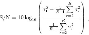
can be regarded as a signal trace. The S/N of the ![]() th CMP can therefore
be estimated as
th CMP can therefore
be estimated as
The second example is a 2D synthetic model
that includes four reflectors. Synthetic data are
generated with Kirchhoff modeling. The peak of
the data set is one and Gaussian random noise
with distribution
![]() is added.
We show the results of stacking one CMP gather
(Figure 3a) by three methods in
Figure 3c-e.
Compared to other methods, our method is the
most effective in denoising.
is added.
We show the results of stacking one CMP gather
(Figure 3a) by three methods in
Figure 3c-e.
Compared to other methods, our method is the
most effective in denoising.

|
|---|
|
onestack1
Figure 3. (a) One CMP gather from synthetic data set. (b) NMO-corrected gather. (c) Result of conventional equal-weight stacking. (d) Result of LMO-based weighted stacking. (e) Result of local-correlation weighted stacking. |
|
|
The stacked profile of all CMP gathers is shown in Figure 4. We use equation 12 to compute the S/N of the stacked profile (Figure 4). The S/Ns of three methods are 7.1, 9.6, 10.9 dB, respectively. Noise is attenuated more effectively in the stacking result using local correlation (Figure 4c).

|
|---|
|
stackss
Figure 4. Comparison among three stacking methods including all synthetic CMP gathers. (a) Conventional equal-weight stacking (S/N=7.1). (b) LMO-based weighted stacking (S/N=9.6). (c) Local-correlation weighted stacking (S/N=10.9). |
|
|
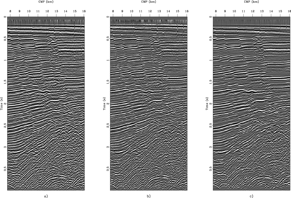
The third example involves a historic 2D line
from the Gulf of Mexico (Claerbout, 2005). The
stacked sections, using three different methods,
are shown in Figure 5. Figure 6 shows the local
correlation cube between prestack and reference
traces. Similar cubes have been used in multicomponent
seismic image registration (Fomel et al., 2005; Fomel, 2007a) and time-lapse image
registration (Fomel and Jin, 2007). For synthetic
data, the exact desired stacked section can be calculated
by stacking prestack traces without any
noise. But for field data, the S/N is difficult to estimate
using equation 12. We therefore use singular
value decomposition (SVD) Andrews and Patterson (1976) to evaluate different stacking
methods. The SVD of stacked section matrix gives
The diagonal elements ![]() of
of ![]() are the singular values of
are the singular values of
![]() . The S/N can be estimated as (Peterson and DeGroat, 1988; Grion and Mazzotti, 1998; Freire and Ulrych, 1988)
. The S/N can be estimated as (Peterson and DeGroat, 1988; Grion and Mazzotti, 1998; Freire and Ulrych, 1988)
where ![]() is the number of all singular values. The S/Ns of stacked
sections resulting from three stacking methods are, respectively,
27.4, 29.2, and 33.9 dB. Comparing Figure 5a-c, we can find also
that random noise is attenuated and coherent reflections are enhanced
better using local correlation (e.g., 0.5-1.5-s range).
is the number of all singular values. The S/Ns of stacked
sections resulting from three stacking methods are, respectively,
27.4, 29.2, and 33.9 dB. Comparing Figure 5a-c, we can find also
that random noise is attenuated and coherent reflections are enhanced
better using local correlation (e.g., 0.5-1.5-s range).
|
|---|
|
field
Figure 5. Results of (a) conventional equal-weight stacking (S/N=27.4), (b) LMO-based weighted stacking (S/N=29.2) and (c) local-correlation weighted stacking (S/N=33.9). |
|
|

|
|---|
|
weight
Figure 6. Local correlation cube of the field-data example. |
|
|
|
|
|
|
Stacking seismic data using local correlation |
![\begin{displaymath}
\textrm{S/N}_j = 10 \log_{10} \left(\frac{\displaystyle\sum...
...)]}{\displaystyle\sum_t[d_j(t)-\bar{a}_j(t)]^2} \right) \;,
\end{displaymath}](img54.png)