|
|
|
|
Least-squares path-summation diffraction imaging using sparsity constraints |
Next: Objective function Up: Method Previous: Method
|
|
|
|
Least-squares path-summation diffraction imaging using sparsity constraints |
Landa et al. (2006) present a path-integral imaging approach, which
does not require knowledge of a velocity distribution in the subsurface.
Burnett et al. (2011) adopt this approach and employ the principle of
diffraction apex stationarity under migration velocity perturbation (Novais et al., 2006) to evaluate
the diffraction path-summation migration integral![]() through stacking of constant migration
velocity images. The images are generated by velocity continuation (VC)
technique, which corresponds to the following transformation in the Fourier domain (Fomel, 2003):
through stacking of constant migration
velocity images. The images are generated by velocity continuation (VC)
technique, which corresponds to the following transformation in the Fourier domain (Fomel, 2003):
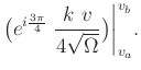
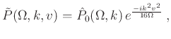
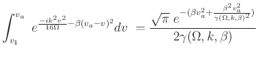
In our previous work (Merzlikin and Fomel, 2017a), we derived analytical formulae for path-summation integral evaluation based on the continuity of VC transformation with respect to velocity: stacking of constant migration velocity images is replaced by a direct integral expression. Analytical formulae allow us to treat path-summation imaging workflow as a simple filter in the frequency-wavenumber domain. Here, we extend Gaussian weighting path-summation migration scheme (Merzlikin and Fomel, 2017a) to account for variable velocity in the subsurface: we design a weighting function, which has a flat region in the middle and has a Gaussian decay for the tail-elimination region as opposed to a curve with one most probable velocity value in regular Gaussian weighting path-summation integral. The following expression describes path-summation integral with Gaussian tapering:
|
|
|
|
Least-squares path-summation diffraction imaging using sparsity constraints |

 erfi
erfi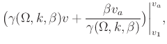
 erfi
erfi