|
|
|
|
Least-squares path-summation diffraction imaging using sparsity constraints |
Next: Field data example Up: Merzlikin et al.: Least-squares Previous: Workflow
|
|
|
|
Least-squares path-summation diffraction imaging using sparsity constraints |
We use the following synthetic to test the proposed chain-inversion
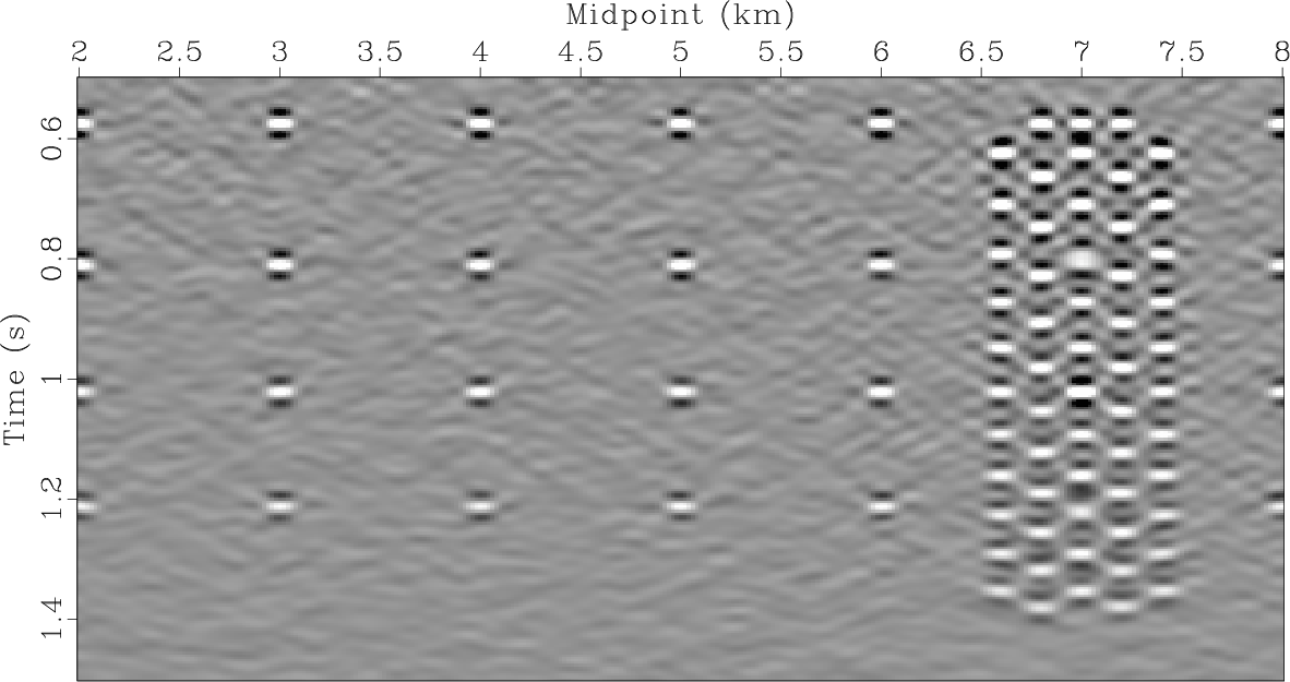
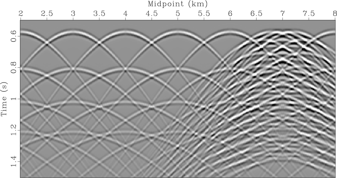
approach. Figure 2 shows a zero-offset modeling result in a
medium with a constant vertical gradient of velocity. The starting velocity at the surface corresponds to
![]() . The section contains reflections with various dips, several layers of sparse diffractions and an area,
in which the density of scatterers is increased (towards the right edge of the synthetic).
Random noise with a 30% magnitude of that of the diffractions and filtered to the signal frequency band is
added to the section.
. The section contains reflections with various dips, several layers of sparse diffractions and an area,
in which the density of scatterers is increased (towards the right edge of the synthetic).
Random noise with a 30% magnitude of that of the diffractions and filtered to the signal frequency band is
added to the section.

|
|---|
|
diffr-irefl-n
Figure 2. Modeled synthetic zero-offset section with reflections, diffractions and noise. |
|
|
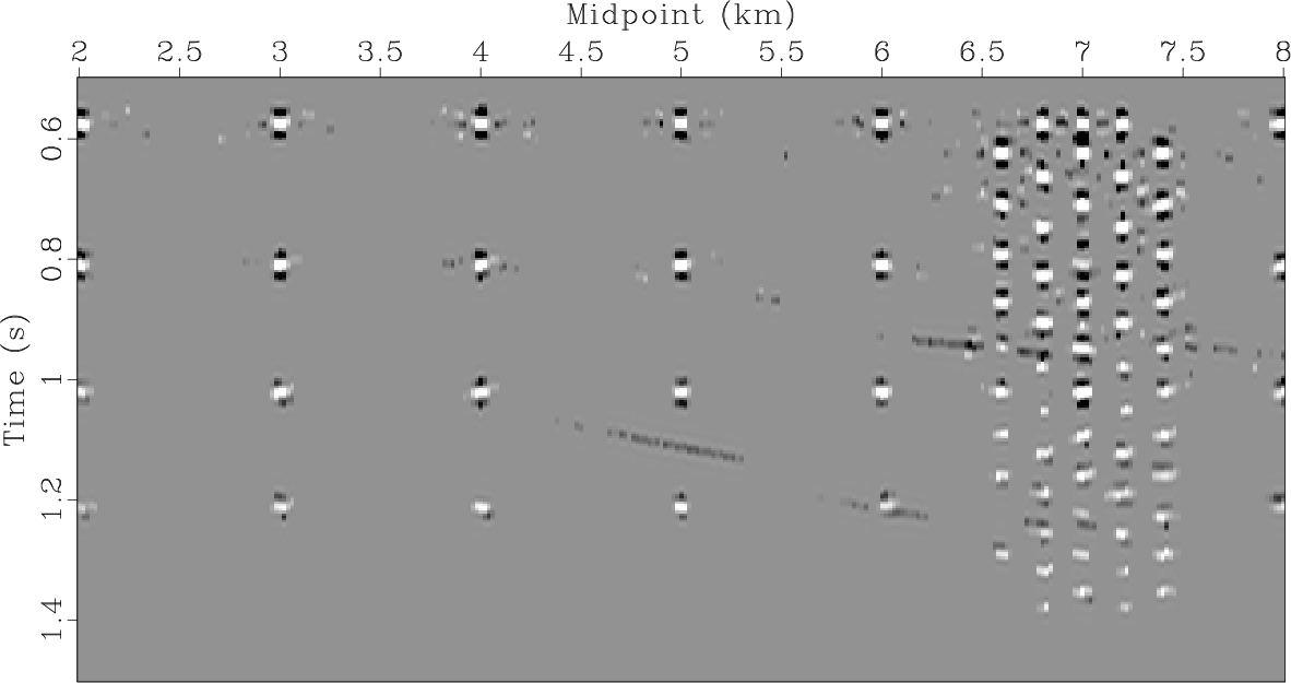
First, we illustrate the advantage of misfit minimization with a diffraction probability weight using
the same synthetic (Figure 2) but with no reflections (Figure 3a)
in order to compare its performance with least-squares Kirchhoff migration. Reflection/diffraction separation is
considered further. Figure 4a shows the result of least-squares Kirchhoff migration (equation 5) with no regularization. Noise leakage into
the diffraction image domain can be easily noticed. The result of path-summation migration applied to the zero-offset synthetic data (Figure 3a)
is shown in Figure 3b. Path-summation migration image can provide us
with a probability of a scatterer at a certain sample location. We employ this information by weighting the misfit term in the
equation 5 by the path-summation migration operator (
![]() ), which forces the misfit minimization only at probable diffraction
locations. No PWD (
), which forces the misfit minimization only at probable diffraction
locations. No PWD (
![]() ) is required to emphasize diffractions since there are no reflections.
Since the input contains diffractions only we need only one model for diffractions
) is required to emphasize diffractions since there are no reflections.
Since the input contains diffractions only we need only one model for diffractions
![]() . No reflection model is considered.
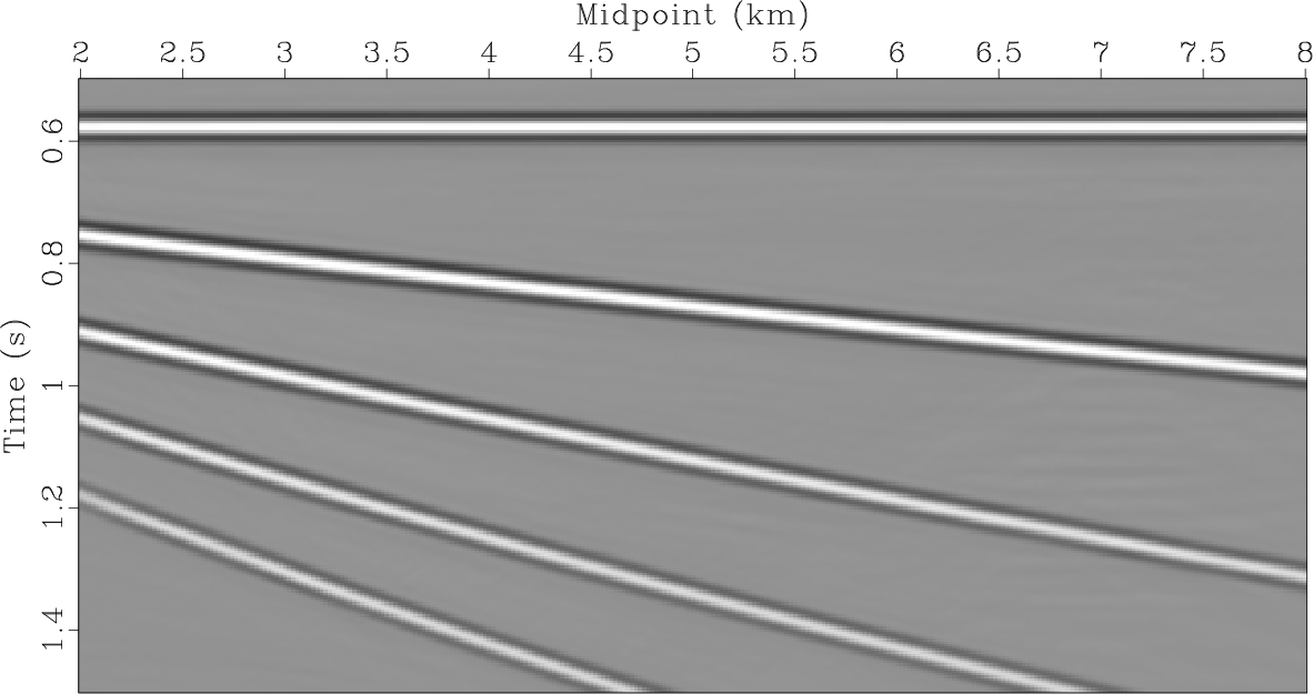
Figure 4b shows the result of least-squares Kirchhoff migration with a misfit
weighted by path-summation integral filter. No regularization has been applied. It can be seen
that weighted minimization reduces high frequency artifacts. Path-summation integral operator emphasizes
diffraction apexes remaining stationary under migration velocity perturbation. It acts as a low-frequency
filter guiding the inversion towards probable scatterers locations. Indeed, lower frequency content is noticeable
and diffractions are more visible on the result of weighted minimization (Figure 4b) than on the “conventional" least-squares Kirchhoff migration image
(Figure 4a). Incorporation of sparsity constraints will remove high
frequency artifacts from the least-squares Kirchhoff migration image and will reduce the area
corresponding to a diffraction location in a weighted minimization result. Here, regularization is disabled to show the effectiveness
of path-summation operator misfit weighting and avert the subjective choice of a regularization parameter, which will influence the results
and make their unbiased comparison harder.
. No reflection model is considered.
Figure 4b shows the result of least-squares Kirchhoff migration with a misfit
weighted by path-summation integral filter. No regularization has been applied. It can be seen
that weighted minimization reduces high frequency artifacts. Path-summation integral operator emphasizes
diffraction apexes remaining stationary under migration velocity perturbation. It acts as a low-frequency
filter guiding the inversion towards probable scatterers locations. Indeed, lower frequency content is noticeable
and diffractions are more visible on the result of weighted minimization (Figure 4b) than on the “conventional" least-squares Kirchhoff migration image
(Figure 4a). Incorporation of sparsity constraints will remove high
frequency artifacts from the least-squares Kirchhoff migration image and will reduce the area
corresponding to a diffraction location in a weighted minimization result. Here, regularization is disabled to show the effectiveness
of path-summation operator misfit weighting and avert the subjective choice of a regularization parameter, which will influence the results
and make their unbiased comparison harder.


|
|---|
|
diffr-n,idpi-mig2-n
Figure 3. (a) Diffraction and noise components of the synthetic shown in Figure 2; (b) path-summation migration applied to zero-offset synthetic with no reflections (Figure 3a). |
|
|

|
|---|
|
lsq-mig2,lsq-pi
Figure 4. Imaging of diffractions with noise (Figure 3a) using (a) least-squares Kirchhoff migration; (b) least-squares Kirchhoff migration weighted by diffraction probability (see text for details); no regularization applied. Both images are generated with the same number of iterations. |
|
|
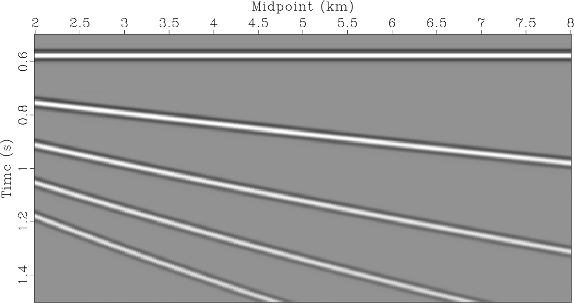
We then apply the proposed workflow to the synthetic containing all the components with regularization enabled. First, we
estimate slopes of the dominant events, which are associated with reflections, in the data and image domains. We then generate
the data for the first inversion cascade (Figure 5a): zero-offset section (Figure 2) is weighted
by PWD (
![]() ) and path-summation integral filter (
) and path-summation integral filter (
![]() ). We run
). We run ![]() outer iterations and
outer iterations and ![]() inner iterations.
Convergence curves are shown in Figure 6.
The results of the first inversion are shown in Figure 5.
Although subtle reflection remainders are present (e.g.
inner iterations.
Convergence curves are shown in Figure 6.
The results of the first inversion are shown in Figure 5.
Although subtle reflection remainders are present (e.g.
![]() TWTT (two-way travel time) and
TWTT (two-way travel time) and
![]() distance) the majority of diffracted energy has been extracted with high accuracy.
distance) the majority of diffracted energy has been extracted with high accuracy.


|
|---|
|
pi-w-pwd-s,refly-w-pwd-s,diffry-w-pwd-s
Figure 5. (a) Zero-offset section weighted by path-summation integral operator ( |
|
|

|
|---|
|
convergence-synth
Figure 6. Convergence of the inversion with PWD (equation 6): left - residual in the data space; right - difference between consecutive models. |
|
|
To reduce these remainders and restore reflections trapped in the null space of the “chain" of operators we run the second inversion
cascade with no PWD. First, we generate the data to be fit (Figure 7a): PWD is disabled and
only path-summation integral operator is used to weight the misfit. The result of the first inversion cascade (Figure 5)
is used as the starting model for the second inversion. We run ![]() outer iterations and
outer iterations and ![]() inner to restore reflections and reduce the reflection-diffraction crosstalk. Orthogonalization
is required. Figure 8 shows the updates to reflections and diffractions after the first external iteration
of the second inversion (equation 8). Orthogonalization is applied to remove reflections from the diffraction image update: it can be seen that reflections
in the update are significantly stronger than diffractions and are hard to suppress with thresholding only. Orthogonalization significantly reduces the energy of reflections
and diffraction-related update becomes more visible (Figure 8b). The orthogonalized update is then added to diffraction model followed by shaping regularization.
Reflection and diffraction images shown in Figure 7 are generated.
Reflections are recovered from the null space introduced by PWD. Crosstalk is reduced (Figure 7c: e.g.
inner to restore reflections and reduce the reflection-diffraction crosstalk. Orthogonalization
is required. Figure 8 shows the updates to reflections and diffractions after the first external iteration
of the second inversion (equation 8). Orthogonalization is applied to remove reflections from the diffraction image update: it can be seen that reflections
in the update are significantly stronger than diffractions and are hard to suppress with thresholding only. Orthogonalization significantly reduces the energy of reflections
and diffraction-related update becomes more visible (Figure 8b). The orthogonalized update is then added to diffraction model followed by shaping regularization.
Reflection and diffraction images shown in Figure 7 are generated.
Reflections are recovered from the null space introduced by PWD. Crosstalk is reduced (Figure 7c: e.g.
![]() TWTT and
TWTT and
![]() distance).
Different choice of regularization parameters including the balance between the numbers of internal and external iterations in the first and
second inversions can be tweaked to improve the results even more.
distance).
Different choice of regularization parameters including the balance between the numbers of internal and external iterations in the first and
second inversions can be tweaked to improve the results even more.


|
|---|
|
pi-n-pwd-s,refly-n-pwd-s,diffry-n-pwd-s
Figure 7. (a) Zero-offset section weighted by path-summation integral operator ( |
|
|


|
|---|
|
update-b4-diffr-synth,update-a4-diffr-synth
Figure 8. Updates to the model: (a) update to diffractions before orthogonalization (equation 12; reflections have the same update); (b) update to diffractions after orthogonalization: reflections are suppressed and diffraction-related update is more visible. |
|
|
We then run the inversions (equations 10 and 11) to restore high wavenumbers with PWD and path-summation integral operators disabled. For diffraction-only recovery (equation 11) besides using the starting model from the second inversion as an additional regularization the model is masked by the locations of the diffractors. This mask can easily be created from the diffraction image generated as the output of the second inversion cascade (Figure 7c). Figure 9 show reflection and diffraction components restored by the inversions, which were generated by applying Kirchhoff forward modeling operator to reflectivity and diffractivity output by wavenumber restoration inversions (equations 10 and 11). We then subtract recovered reflections and diffractions from the input data to generate the noise estimate. Noise and diffractions are plotted with the same gain. Although the noise section contains some diffracted energy, the approach is highly effective. We then compare the results with the true components used to generate the synthetic. High correlation between the restored and the “true" components of the synthetic also supports high accuracy of the workflow. Signal and noise orthogonalization helps to account for amplitude differences between “true" and restored diffractions (Figure 9c and 9d): although high restoration quality is achieved subtle amplitude differences can be noticed. Since diffraction shapes are restored this energy can be brought from the noise section back to the diffraction image domain by measuring the similarity between the corresponding components.
Simultaneous inversion for both reflections and diffractions allows to account for the crosstalk between the components and thus improves the confidence of scatterer position identification. We proceed with the workflow application to the field data example.


|
|---|
|
rs-s,t-rs,ds-s,t-ds,n-s,t-n
Figure 9. (a) Restored reflections, (b) true reflections, (c) restored diffractions, (d) true diffractions, (e) restored noise, (f) true noise |
|
|
|
|
|
|
Least-squares path-summation diffraction imaging using sparsity constraints |