next up previous [pdf]

Next: Frequency attenuation estimation Up: Application Previous: Application

Synthetic and field data test

To test our method, we generated a wavelet composed of three Ricker wavelets with peak frequencies of 10, 20, and 50 Hz (Figure 1.) Applying a separable nonlinear least-squares estimation, we estimated peak frequencies at $ 9.999$ , $ 19.999$ , and $ 49.995$ Hz. The residual sum of squares equals approximately $ 10^{-7}$ after $ 50$ iterations. The estimation fits the wavelet spectrum accurately, as shown in Figure 1. Generally speaking, the more terms we use to fit the data, the better fitting result we may obtain. However, it is geological reasoning, not statistical factors that determines how many terms should be used in the model. A real data example, shows that spectral recomposition works well for field data (Figure 2). In this case, the estimated peak frequencies are approximately 15 Hz, 31 Hz, and 43 Hz.

rk
rk
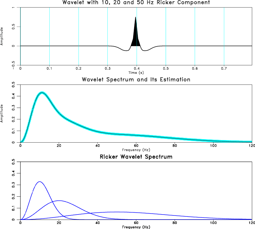
Figure 1.
(a) A wavelet composed of 10, 20 and 50 Hz Ricker components. (b) The estimated wavelet spectrum components are plotted individually. The estimated peak frequencies of these components are 9.999, 19.999 and 49.995 Hz. (c) We computed and estimated the spectrum of the wavelet in (a). Spectral recomposition result (in green) fits the spectrum (in black) very well.
[pdf] [png] [scons]

recomp
recomp
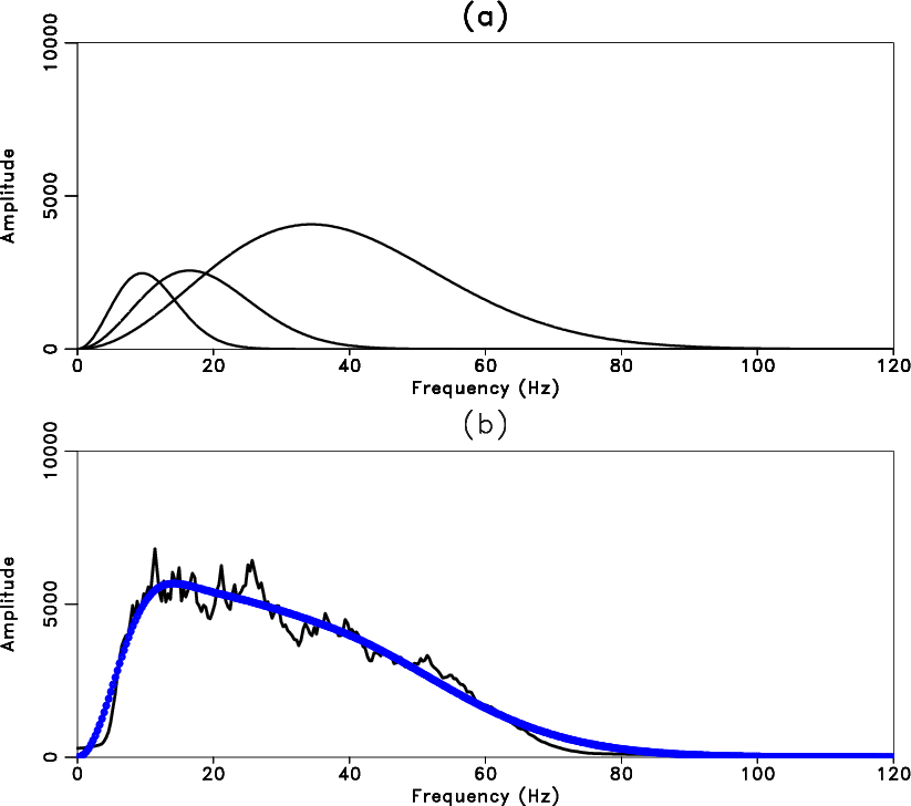
Figure 2.
(a) Spectra of ricker wavelet components. Each spectral component is well separated, probably indicating different geological factors. (b) Spectral recomposition result (in blue) fits the seismic spectrum (in black) well.
[pdf] [png] [scons]


next up previous [pdf]

Next: Frequency attenuation estimation Up: Application Previous: Application

2013-08-19