Deblending using a space-varying median filter

Implementation steps of SVMF

Unlike 2D signal-processing field, where the signal is multi-dimensionally coherent, geophysical data is energy-focusing only spatially . Due to the temporal sparseness of the property, the useful signal takes a spike-like form. This spatial coherence makes it necessary to take a conventional MF along the spatial direction. Besides, the local slope of an event should be small in order to ensure a small energy loss. In the case of dipping events, a multidimensional MF can be used as a substitute of the conventional MF (Huo et al., 2012), or in the other way, one can let the length of filtering window be smaller. However, reducing the length of the filtering window reduces the ability of an MF to remove spiky noise commensurately. Balancing removal of spiky noise while minimizing energy loss is always a compromise. The SVMF utilizes a two-step strategy: first, use MF to coarsely filter the data and obtain a calculation of signal reliability (SR), and then use an adaptive MF filter with window length varying according to the difference with respect to SR. The initial constant filter length is chosen so that most of the blending noise can be removed regardless of a small loss of useful signals. Empirically, the initial filter length can be between 7 and 11. In both steps, the MF is implemented along the spatial direction. Figure 3 shows a filtering comparison using different kinds of filters. The data is similar to that used in Huo et al. (2012). To be effective, MF should only be implemented along the spatial direction, and by using SVMF, the dipping events can be preserved to a large extent. The algorithms steps of SVMF can be summarized as follows:

1. Apply the first MF using constant filter length.
2. Compute the SR map by computing the local similarity between the data initially filtered using MF and the original seismic data.
3. Compute the map of variable filter length.
4. Apply the secondary MF using the variable filter length.

huos,huos-tmf,huos-xmf,huos-svmf
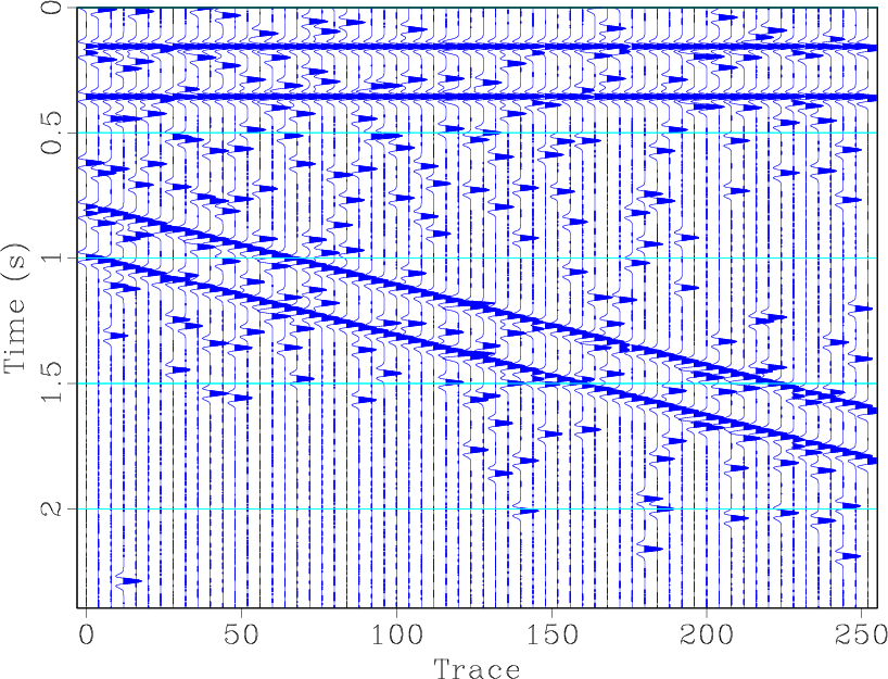
Figure 3. Comparison of different kinds of MF. (a) Original noisy data. (b) Implementing MF along temporal direction. (c) Implementing MF along spatial direction. (d) Implementing SVMF with two-step MF along spatial direction.

Deblending using a space-varying median filter