Time-frequency analysis of seismic data using synchrosqueezing wavelet transform

Field examples

data,lowf,higf
Figure 2. (a) Input data. (a) Frequency slice corresponding to 30 Hz. (b) Frequency slice corresponding to 60 Hz.

timefreq-st,timefreq,pp-tfsswt
Figure 3. (a) Time-frequency map of the S transform. (b) Time-frequency map using local attributes. (c) Time-frequency map using the synchrosqueezing wavelet transform.

The first field data (Figure 2a) is a land seismic survey used previously by (Fomel, 2013). We extract two frequency slices (30 Hz and 60 Hz) from the TF decomposed result and show them in Figures 2b and 2c. It's obvious that the high-frequency slice has some anomalies pointed out by the labels, which may comes from the high-frequency attenuation because of the trapped oil & gas. The results are consistent from that found by Fomel (2013) using a different technique. The TF cube of the real data corresponding to three different TF analysis approaches are shown in Figure 3. The TF map of the S transform seems blurs together. While the local attributes based TF analysis can have good time resolution, the SSWT can get a better result. The deep-layer of the TF cube show coherent frequency components, indicating the potential week signal which can not be sensed visually or by the other two TF analysis approaches. The detection of deep-layer week signal is significant because these weak signals usually indicate the existence of layers that has obvious impedance difference compared with their overburden layers. Especially when the detected signals are mainly existing in the low frequency band, the detection will indicate the existence of residual oil&gas traps.

old-1
Figure 4. Field data example for detecting low frequency anomalies.

s1,s2,s3,tf-s,l1,l2,l3,tf-l,ss1,ss2,ss3,tf-ss
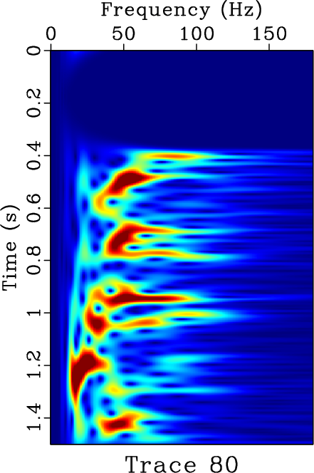
Figure 5. (a)-(c) Frequency slices of 20Hz, 40Hz, and 60 Hz, using the S transform. (d) Time-frequency spectral map using the S transform for 80th trace of the seismic profile shown in Figure 4. (e)-(g) Frequency slices of 20Hz, 40Hz, and 60 Hz, using the local-attributes related TF decomposition. (h) Time-frequency spectral map using the local-attributes related TF decomposition for 80th trace of the seismic profile shown in Figure 4. (i)-(k) Frequency slices of 20Hz, 40Hz, and 60 Hz, using the SSWT. (l) Time-frequency spectral map using the SSWT for 80th trace of the seismic profile shown in Figure 4.

The second field data example is a post-stack field data set, which is also used in the literature by Liu et al. (2011). The data is shown in Figure 4. In this example, we extract three constant-frequency slices corresponding to 20Hz, 40Hz, and 60 Hz, using three different TF decomposition approaches: TF decomposition using the S transform, TF decomposition using local attributes and TF decomposition using the SSWT. We also extract a time-frequency spectral map for the 80th trace in the field data shown in Figure 4. All the constant-frequency slices and TF spectral map are shown in Figure 5.

From the constant-frequency slices shown in Figure 5, we can observe that the S transform has the lowest time resolution, followed by the local-attributes related TF decomposition. The constant-frequency slices and the TF spectral map from the SSWT both show that the TF decomposed results have the largest resolution both in time and frequency. From the TF spectral map, the S transform has a slightly lower frequency resolution. By the SSWT based TF decomposition, we can detect several low-frequency anomalies. In this example, we just emphasize four clearest anormalies, and point out them by four frame boxes with different colors. To better illustrate the result, let us first focus on Figure 5i. The four frame boxes pointed out four strong-amplitude areas, which do not show in its corresponding higher-frequency slices. Thus, these four anomalies may indicate potential oil&gas traps with high probability. Even though from the constant-frequency slices using other two approaches have more or less some anomalies, these anomalies are not very easy to detect. Some highly-potential sweet spots have been lost by using the other two approaches, e.g., area pointed out by the four frame boxes. The best strategy for implementing the SSWT based TF decomposition onto the interpretation for subsurface phenomenons is to combine the SSWT based TF decomposition with the conventional approaches. While the SSWT based TF decomposition can point out the potential anomalies with high fidelity, a more convincing conclusion can be obtained by considering the results from the other approaches.

Time-frequency analysis of seismic data using synchrosqueezing wavelet transform