 |
 |
 |
 | Time-to-depth conversion and seismic velocity estimation using time-migration velocity |  |
![[pdf]](icons/pdf.png) |
Next: Seismic Velocity
Up: Cameron, Fomel, Sethian: Velocity
Previous: Introduction
Kirchhoff prestack time migration is commonly based on the following
travel time approximation (Yilmaz, 2001). Let
 be a
source,
be a
source,
 be a receiver, and
 be the reflection
subsurface point. Then the total travel time from
to
and from
to
is approximated as
be the reflection
subsurface point. Then the total travel time from
to
and from
to
is approximated as
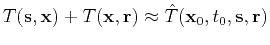 |
(1) |
where
 and
and  are effective parameters
of the subsurface point
. The approximation
are effective parameters
of the subsurface point
. The approximation  usually takes the form of the double-square-root equation
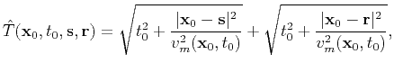 |
(2) |
where
and
are the escape location and the travel
time of the image ray (Hubral, 1977) from the subsurface point
. Regarding this approximation, let us list four cases
depending on the seismic velocity  and the dimension of the
problem:
and the dimension of the
problem:
- 2-D and 3-D, velocity
is constant.
- Equation 2 is exact, and
 .
.
- 2-D and 3-D, velocity
depends only on the depth
 .
.
- Equation 2 is a consequence of the truncated Taylor expansion
for the travel time around the surface point
.
Velocity
 depends only on
and is the root-mean-square velocity:
depends only on
and is the root-mean-square velocity:
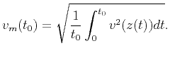 |
(3) |
In this case, the Dix inversion formula (Dix, 1955) is exact. We
formally define the Dix velocity
 by inverting
equation 3, as follows:
by inverting
equation 3, as follows:
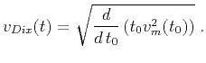 |
(4) |
- 2-D, velocity is arbitrary.
- Equation 2 is a consequence of the truncated Taylor expansion
for the travel time around the surface point
 .
Velocity
.
Velocity
 is a certain kind of mean velocity, and
we establish its exact meaning in the next section.
is a certain kind of mean velocity, and
we establish its exact meaning in the next section.
- 3-D, velocity is arbitrary.
- Equation 2 is heuristic and is not a consequence of the
truncated Taylor expansion. In order to write an analog of
travel time approximation 2 for 3-D, we use the
relation (Hubral and Krey, 1980)
![$\displaystyle \tensor{\Gamma}=[v(\mathbf{x}_0)\tensor{R}(\mathbf{x}_0,t_0)]^{-1},$](img24.png) |
(5) |
where
 is the matrix
of the second derivatives of the travel times
from a subsurface point
to the surface,
is the matrix
of the second derivatives of the travel times
from a subsurface point
to the surface,
 is the matrix of radii of curvature of the emerging wave front
from the point source
, and
is the matrix of radii of curvature of the emerging wave front
from the point source
, and
 is
the velocity at the surface point
.
For convenience, we prefer to deal with matrix
is
the velocity at the surface point
.
For convenience, we prefer to deal with matrix
 ,
which, according to equation 5 is
,
which, according to equation 5 is
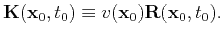 |
(6) |
The travel time approximation for 3-D implied by the Taylor expansion is
The entries of the matrix
 have dimension of squared velocity and can be chosen optimally in the
process of time migration.
It is possible to show, however, that one needs only the values of
have dimension of squared velocity and can be chosen optimally in the
process of time migration.
It is possible to show, however, that one needs only the values of
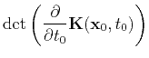 |
(8) |
to perform the inversion. This means that the conventional 3-D
prestack time migration with traveltime approximation 2
provides sufficient input for our inversion procedure in 3-D. The
determinant in equation 8 is well approximated by the
square of the Dix velocity obtained from the 3-D prestack time
migration using the approximation given by equation 2.
One can employ more complex and accurate approximations than the double-square-root equations 2 and 7, i.e. the shifted hyperbola approximation
(Siliqi and Bousquié, 2000). However, other known approximations also involve parameters equivalent to
or
 .
.
|
|
|
|
| Time-to-depth conversion and seismic velocity estimation using time-migration velocity | |
|
Next: Seismic Velocity
Up: Cameron, Fomel, Sethian: Velocity
Previous: Introduction
2013-07-26
![$\displaystyle \sqrt{t_0^2+t_0(\mathbf{x}_0-\mathbf{s})^T
[\tensor{K}(\mathbf{x}_0,t_0)]^{-1}(\mathbf{x}_0-\mathbf{s})}$](img32.png)
![$\displaystyle \sqrt{t_0^2+t_0(\mathbf{x}_0-\mathbf{r})^T
[\tensor{K}(\mathbf{x}_0,t_0)]^{-1}(\mathbf{x}_0-\mathbf{r})}.$](img34.png)